%%capture

import tqdm
from IPython import get_ipython

install_packages = "google.colab" in str(get_ipython())
if install_packages:
    !pip install zfit hepstats
Introduction to zfit - Extended#
In this notebook, we will have a walk through the main components of zfit and their features. Especially the extensive model building part will be discussed separately. zfit consists of 5 mostly independent parts. Other libraries can rely on these parts to do plotting or statistical inference, such as hepstats does. Therefore, we will discuss two libraries in this tutorial: zfit to build models, data and a loss, minimize it and get a fit result and hepstats, to use the loss we built here and do inference.
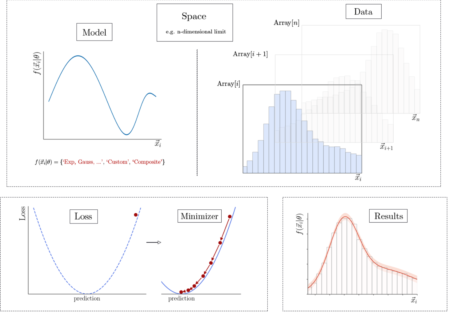
Data - Extended#
This component in general plays a minor role in zfit: it is mostly to provide a unified interface for data.
Most places do not require the use of zfit data and pandas/array-like or hist objects can be used directly (in case of ambiguity, an error is raised)
Preprocessing (apart from a rectangular cut) is therefore not part of zfit and should be done beforehand. Python offers many great possibilities to do so (e.g. Pandas).
zfit Data can load data from various sources, most notably from Numpy, Pandas DataFrame and ROOT (using uproot) for unbinned data as well as hist histograms for binned data. It is also possible, for convenience, to convert back directly with to_pandas or to_hist. The explicity constructors are named from_numpy, from_root etc.
import matplotlib.pyplot as plt
import numpy as np
import zfit
# znp is a subset of numpy functions with a numpy-like interface but using actually the zfit backend (currently TF)
import zfit.z.numpy as znp
import zfit_physics as zphys
from zfit import z
A Data needs not only the data itself but also the observables: the human readable string identifiers of the axes (corresponding to “columns” of a Pandas DataFrame). It is convenient to define the Space not only with the observable but also with a limit: this can directly be re-used as the normalization range in the PDF.
First, let’s define our observables
obs = zfit.Space('obs1', -5, 10, label="Observable 1") # label is optional
This Space has limits. Next to the effect of handling the observables, we can also play with the limits: multiple Spaces can be added to provide disconnected ranges. More importantly, Space offers functionality (currently, add a .v1 in front of all these functions for forward compatibility, i.e. obs.v1.limits):
limits: the
(lower, upper)limits as a tuple of 1D arraysvolume: calculate the area/volume (e.g. distance between upper and lower)
labels: Different labels of the spaces
inside(): return a boolean Tensor corresponding to whether the value is inside the
Spacefilter(): filter the input values to only return the one inside
size_normal = 10000
data_normal_np = np.random.normal(size=size_normal, scale=2)

data_normal = zfit.Data(data=data_normal_np, obs=obs)
data_normal = zfit.data.from_numpy(obs=obs, array=data_normal_np)  # or using an explicit constructor with more options
The main functionality is
nevents: attribute that returns the number of events in the object
space: a
Spacethat defines the limits of the data; if outside, the data will be cutn_obs: defines the number of dimensions in the dataset
with_obs: returns a subset of the dataset with only the given obs
weights: event based weights
Furthermore, value returns a Tensor with shape (nevents, n_obs).
To retrieve values, in general z.unstack_x(data) should be used; this returns a single Tensor with shape (nevents) or a list of tensors if n_obs is larger then 1.
print(
    f"We have {data_normal.nevents} events in our dataset with the minimum of {np.min(data_normal.unstack_x())}")  # remember! The obs cut out some of the data
We have 9944 events in our dataset with the minimum of -4.970360779950905
data_normal.n_obs
1
Model - Extended#
Building models is by far the largest part of zfit. We will therefore cover an essential part, the possibility to build custom models, in an extra chapter. Let’s start out with the idea that you define your parameters and your observable space; the latter is the expected input data.
There are two types of models in zfit:
functions, which are rather simple and “underdeveloped”; their usage is often not required.
PDF that are function which are normalized (over a specified range); this is the main model and is what we gonna use throughout the tutorials.
A PDF is defined by
where a and b define the normalization range (norm), over which (by inserting into the above definition) the integral of the PDF is unity.
zfit has a modular approach to things and this is also true for models. While the normalization itself (e.g. what are parameters, what is normalized data) will already be pre-defined in the model, models are composed of functions that are transparently called inside. For example, a Gaussian would usually be implemented by writing a Python function def gauss(x, mu, sigma), which does not care about the normalization and then be wrapped in a PDF, where the normalization and what is a parameter is defined.
In principle, we can go far by using simply functions (e.g. TensorFlowAnalysis/AmpliTF by Anton Poluektov uses this approach quite successfully for Amplitude Analysis), but this design has limitations for a more general fitting library such as zfit (or even TensorWaves, being built on top of AmpliTF). The main thing is to keep track of the different ordering of the data and parameters, especially the dependencies.
Let’s create a simple Gaussian PDF. We already defined the Space for the data before, now we only need the parameters. This are a different object than a Space.
Parameter - Extended#
A Parameter (there are different kinds actually, more on that later) takes the following arguments as input:
Parameter(human readable name, initial value[, lower limit, upper limit]) where the limits are recommended but not mandatory. Furthermore, step_size can be given (which is useful to be around the given uncertainty, e.g. for large yields or small values it can help a lot to set this). Also, a floating argument is supported, indicating whether the parameter is allowed to float in the fit or not (just omitting the limits does not make a parameter constant).
The name of the parameter identifies it; therefore, while multiple parameters with the same name can exist, they cannot exist inside the same model/loss/function, as they would be ambiguous.
mu = zfit.Parameter('mu', 1, -3, 3, step_size=0.2)
another_mu = zfit.Parameter('mu', 2, -3, 3, step_size=0.2)
sigma_num = zfit.Parameter('sigma42', 1, 0.1, 10, floating=False)
These attributes can be changed:
print(f"sigma is float: {sigma_num.floating}")
sigma_num.floating = True
print(f"sigma is float: {sigma_num.floating}")
sigma is float: False
sigma is float: True
Now we have everything to create a Gaussian PDF:
gauss = zfit.pdf.Gauss(obs=obs, mu=mu, sigma=sigma_num)
Since this holds all the parameters and the observables are well defined, we can retrieve them
gauss.n_obs # dimensions
1
gauss.obs
('obs1',)
gauss.space
<zfit Space obs=('obs1',), axes=(0,), limits=(array([[-5.]]), array([[10.]])), binned=False>
gauss.norm
<zfit Space obs=('obs1',), axes=(0,), limits=(array([[-5.]]), array([[10.]])), binned=False>
As we’ve seen, the obs we defined is the space of Gauss: this acts as the default limits whenever needed (e.g. for sampling). gauss also has a norm, which equals by default as well to the obs given, however, we can explicitly change that with set_norm.
We can also access the parameters of the PDF in two ways, depending on our intention:
either by name (the parameterization name, e.g. mu and sigma, as defined in the Gauss), which is useful if we are interested in the parameter that describes the shape
gauss.params
{'mu': <zfit.Parameter 'mu' floating=True value=1>,
 'sigma': <zfit.Parameter 'sigma42' floating=True value=1>}
or to retrieve all the parameters that the PDF depends on. As this now may sounds trivial, we will see later that models can depend on other models (e.g. sums) and parameters on other parameters. There is one function that automatically retrieves all dependencies, get_params. It takes three arguments to filter:
floating: whether to filter only floating parameters, only non-floating or don’t discriminate
is_yield: if it is a yield, or not a yield, or both
extract_independent: whether to recursively collect all parameters. This, and the explanation for why independent, can be found later on in the
Simultaneoustutorial.
Usually, the default is exactly what we want if we look for all free parameters that this PDF depends on.
gauss.get_params()
OrderedSet([<zfit.Parameter 'mu' floating=True value=1>, <zfit.Parameter 'sigma42' floating=True value=1>])
The difference will also be clear if we e.g. use the same parameter twice:
gauss_only_mu = zfit.pdf.Gauss(obs=obs, mu=mu, sigma=mu)
print(f"params={gauss_only_mu.params}")
print(f"get_params={gauss_only_mu.get_params()}")
params={'mu': <zfit.Parameter 'mu' floating=True value=1>, 'sigma': <zfit.Parameter 'mu' floating=True value=1>}
get_params=OrderedSet([<zfit.Parameter 'mu' floating=True value=1>])
Functionality - Extended#
PDFs provide a few useful methods. The main features of a zfit PDF are:
pdf: the normalized value of the PDF. It takes an argumentnormthat can be set toFalse, in which case we retrieve the unnormalized valueintegrate: given a certain range, the PDF is integrated. Aspdf, it takes anormargument that integrates over the unnormalizedpdfif set toFalsesample: samples from the pdf and returns aDataobject
integral = gauss.integrate(limits=(-1, 3))  # corresponds to 2 sigma integral
integral
<tf.Tensor: shape=(1,), dtype=float64, numpy=array([0.95449974])>
Tensors - Extended#
As we see, many zfit functions return Tensors. This is however no magical thing! If we’re outside of models, than we can always safely convert them to a numpy array by calling zfit.run(...) on it (or any structure containing potentially multiple Tensors). However, this may not even be required often! They can be added just like numpy arrays and interact well with Python and Numpy:
np.sqrt(integral)
array([0.97698502])
They also have shapes, dtypes, can be slices etc. So do not convert them except you need it. More on this can be seen in the talk later on about zfit and TensorFlow 2.0.
sample = gauss.sample(n=1000)  # default space taken as limits
print(f"As DataFrame: {sample.to_pandas()}")
As DataFrame:          obs1
0    1.530794
1    2.899722
2    0.467128
3    0.677786
4    3.369001
..        ...
995  1.219783
996  1.784260
997  1.687152
998  2.861263
999  0.692530

[1000 rows x 1 columns]
print(f"To array-like: {sample.value()[:10]}")
To array-like: [[1.53079376]
 [2.8997219 ]
 [0.46712779]
 [0.6777856 ]
 [3.36900088]
 [1.46192973]
 [0.40327407]
 [1.79201982]
 [0.44717248]
 [1.97754178]]
np.abs(sample['obs1'])[:10] # index like a pandas DataFrame, use like an array
array([1.53079376, 2.8997219 , 0.46712779, 0.6777856 , 3.36900088,
       1.46192973, 0.40327407, 1.79201982, 0.44717248, 1.97754178])
sample.to_numpy().shape # _explicitly_ to numpy (usually not needed)
(1000, 1)
sample.nevents
<tf.Tensor: shape=(), dtype=int32, numpy=1000>
sample.obs
('obs1',)
We see that sample returns also a zfit Data object with the same space as it was sampled in. This can directly be used e.g.
probs = gauss.pdf(sample)
probs[:10]
<tf.Tensor: shape=(10,), dtype=float64, numpy=
array([0.3465218 , 0.06565049, 0.34613897, 0.37876111, 0.02411259,
       0.35857119, 0.33387806, 0.29153762, 0.34240958, 0.24740404])>
NOTE: In case you want to do this repeatedly (e.g. for toy studies), there is a way more efficient way (see later on)
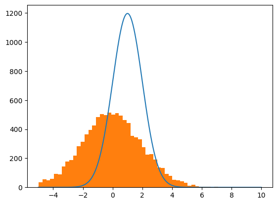
Plotting - Extended#
so far, we have a dataset and a PDF. Before we go for fitting, we can make a plot. This functionality is not extensively covered in zfit, but helper functions exist. It is however simple enough to do it:
def plot_model(model, data, scale=1, plot_data=True):  # we will use scale later on

    nbins = 50

    lower, upper = data.space.v1.limits
    x = znp.linspace(lower, upper, num=1000)  # np.linspace also works
    y = model.pdf(x) * size_normal / nbins * data.space.volume
    y *= scale
    plt.plot(x, y)
    data_plot = zfit.run(z.unstack_x(data))  # we could also use the `to_pandas` method
    if plot_data:
        plt.hist(data_plot, bins=nbins)
plot_model(gauss, data_normal)
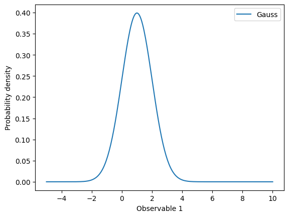
# shortcut to plot pdf
gauss.plot.plotpdf(full=True)  # full plots all the labels, legends as well. False means plot only PDF
<Axes: xlabel='Observable 1', ylabel='Probability density'>
We can of course do better (and will see that later on, continuously improve the plots), but this is quite simple and gives us the full power of matplotlib.
Different models - Extended#
zfit offers a selection of predefined models (and extends with models from zfit-physics that contain physics specific models such as ARGUS shaped models).
print(zfit.pdf.__all__)
['ZPDF', 'BaseBinnedFunctorPDF', 'BaseBinnedPDF', 'BaseFunctor', 'BasePDF', 'Bernstein', 'Beta', 'BifurGauss', 'BinnedFromUnbinnedPDF', 'BinnedSumPDF', 'BinwiseScaleModifier', 'CachedPDF', 'Cauchy', 'Chebyshev', 'Chebyshev2', 'ChiSquared', 'ConditionalPDFV1', 'CrystalBall', 'DoubleCB', 'ExpModGauss', 'Exponential', 'FFTConvPDFV1', 'Gamma', 'Gauss', 'GaussExpTail', 'GaussianKDE1DimV1', 'GeneralizedCB', 'GeneralizedGauss', 'GeneralizedGaussExpTail', 'Hermite', 'HistogramPDF', 'JohnsonSU', 'KDE1DimExact', 'KDE1DimFFT', 'KDE1DimGrid', 'KDE1DimISJ', 'Laguerre', 'Legendre', 'LogNormal', 'Poisson', 'PositivePDF', 'ProductPDF', 'QGauss', 'RecursivePolynomial', 'SimpleFunctorPDF', 'SimplePDF', 'SplineMorphingPDF', 'SplinePDF', 'StudentT', 'SumPDF', 'TruncatedGauss', 'TruncatedPDF', 'UnbinnedFromBinnedPDF', 'Uniform', 'Voigt', 'WrapDistribution']
print(zphys.pdf.__all__)
['Argus', 'CMSShape', 'Cruijff', 'ErfExp', 'Novosibirsk', 'RelativisticBreitWigner', 'Tsallis']
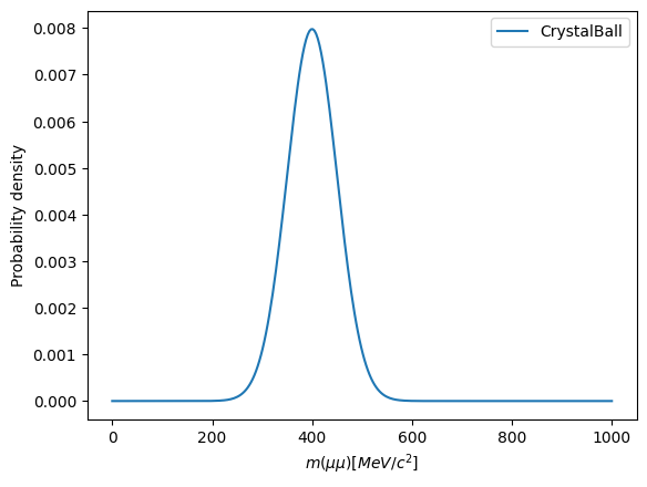
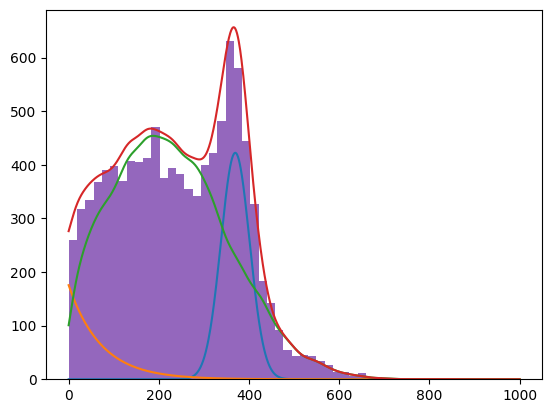
To create a more realistic model, we can build some components for a mass fit with a
signal component: CrystalBall
combinatorial background: Exponential
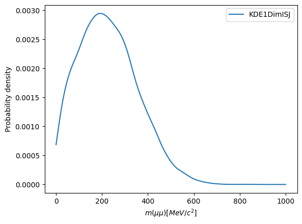
partial reconstructed background on the left: Kernel Density Estimation
mass_obs = zfit.Space('mass', 0, 1000, label=r"$m(\mu\mu) [MeV/c^2]$")
# Signal component

mu_sig = zfit.Parameter('mu_sig', 400, 100, 600)
sigma_sig = zfit.Parameter('sigma_sig', 50, 1, 100)
alpha_sig = zfit.Parameter('alpha_sig', 200, 100, 400, floating=False)  # won't be used in the fit
n_sig = zfit.Parameter('n sig', 4, 0.1, 30, floating=False)
signal = zfit.pdf.CrystalBall(obs=mass_obs, mu=mu_sig, sigma=sigma_sig, alpha=alpha_sig, n=n_sig)
ax = signal.plot.plotpdf()
# combinatorial background

lam = zfit.Parameter('lambda', -0.01, -0.05, -0.00001)
comb_bkg = zfit.pdf.Exponential(lam, obs=mass_obs)
part_reco_data = np.random.normal(loc=200, scale=150, size=20_000)
part_reco_data = zfit.Data.from_numpy(obs=mass_obs,
                                      array=part_reco_data)  # we don't need to do this but now we're sure it's inside the limits

part_reco = zfit.pdf.KDE1DimISJ(obs=mass_obs, data=part_reco_data)
part_reco.plot.plotpdf()
<Axes: xlabel='$m(\\mu\\mu) [MeV/c^2]$', ylabel='Probability density'>
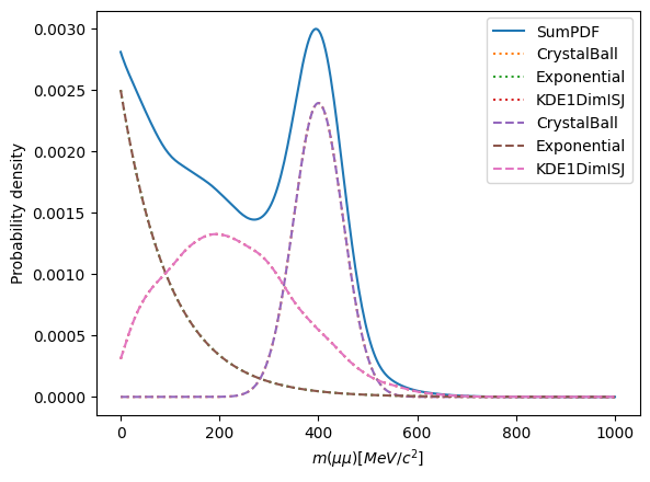
Composing models - Extended#
We can also compose multiple models together. Here we’ll stick to one dimensional models, the extension to multiple dimensions is explained in the “custom models tutorial”.
Here we will use a SumPDF. This takes pdfs and fractions. If we provide n pdfs and:
n - 1 fracs: the nth fraction will be 1 - sum(fracs)
n fracs: no normalization attempt is done by
SumPDf. If the fracs are not implicitly normalized, this can lead to bad fitting behavior if there is a degree of freedom too much
sig_frac = zfit.Parameter('sig_frac', 0.3, 0, 1)
comb_bkg_frac = zfit.Parameter('comb_bkg_frac', 0.25, 0, 1)
model = zfit.pdf.SumPDF([signal, comb_bkg, part_reco], [sig_frac, comb_bkg_frac])
ax = model.plot.plotpdf(full=True)  # just a quick way of plotting the pdf
model.plot.comp.plotpdf(ax=ax, linestyle='--')  # plot the components, only works for pdfs with components to plot
<Axes: xlabel='$m(\\mu\\mu) [MeV/c^2]$', ylabel='Probability density'>
In order to have a corresponding data sample, we can just create one. Since we want to fit to this dataset later on, we will create it with slightly different values. Therefore, we can use the ability of a parameter to be set temporarily to a certain value with
print(f"before: {sig_frac}")
with sig_frac.set_value(0.25):
    print(f"new value: {sig_frac}")
print(f"after 'with': {sig_frac}")
before: sig_frac=0.3
new value: sig_frac=0.25
after 'with': sig_frac=0.3
While this is useful, it does not fully scale up. We can use the zfit.param.set_values helper therefore.
(Sidenote: instead of a list of values, we can also use a FitResult, the given parameters then take the value from the result)
with zfit.param.set_values([mu_sig, sigma_sig, sig_frac, comb_bkg_frac, lam], [370, 34, 0.18, 0.15, -0.006]):
    data = model.sample(n=10000)
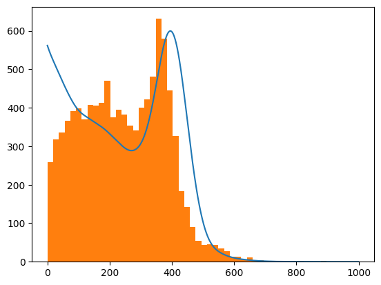
# even better, we directly give the values we want
data = model.sample(n=10000, params={mu_sig: 370, sigma_sig: 34, sig_frac: 0.18, comb_bkg_frac: 0.15, lam: -0.006})
plot_model(model, data);
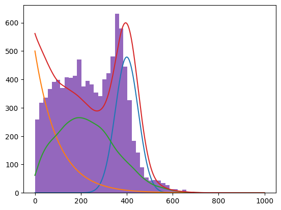
Plotting the components is not difficult now: we can either just plot the pdfs separately (as we still can access them) or in a generalized manner by accessing the pdfs attribute:
def plot_comp_model(model, data):
    for mod, frac in zip(model.pdfs, model.params.values()):
        plot_model(mod, data, scale=frac, plot_data=False)
    plot_model(model, data)
plot_comp_model(model, data)
Now we can add legends etc. Btw, did you notice that actually, the frac params are zfit Parameters? But we just used them as if they were Python scalars and it works.
print(model.params)
{'frac_0': <zfit.Parameter 'sig_frac' floating=True value=0.3>, 'frac_1': <zfit.Parameter 'comb_bkg_frac' floating=True value=0.25>, 'frac_2': <zfit.ComposedParameter 'Composed_autoparam_0' params=[('frac_0', 'sig_frac'), ('frac_1', 'comb_bkg_frac')] value=0.45>}
Extended PDFs - Extended Tutorial#
So far, we have only looked at normalized PDFs that do contain information about the shape but not about the absolute scale. We can make a PDF extended by adding a yield to it.
The behavior of the new, extended PDF does NOT change, any methods we called before will act the same. Only exception, some may require an argument less now. All the methods we used so far will return the same values. What changes is that the flag model.is_extended now returns True. Furthermore, we have now a few more methods that we can use which would have raised an error before:
get_yield: return the yield parameter (notice that the yield is not added to the shape parametersparams)ext_{pdf,integrate}: these methods return the same as the versions used before, however, multiplied by the yieldsampleis still the same, but does not require the argumentnanymore. By default, this will now equal to a poissonian sampled n around the yield.
The SumPDF now does not strictly need fracs anymore: if all input PDFs are extended, the sum will be as well and use the (normalized) yields as fracs
The preferred way to create an extended PDf is to use PDF.create_extended(yield). However, since this relies on copying the PDF (which may does not work for different reasons), there is also a set_yield(yield) method that sets the yield in-place. This won’t lead to ambiguities, as everything is supposed to work the same.
yield_model = zfit.Parameter('yield_model', 10000, 0, 20000, step_size=10)
model_ext = model.create_extended(yield_model)

# or create directly
model_ext = zfit.pdf.SumPDF([signal, comb_bkg, part_reco], fracs=[sig_frac, comb_bkg_frac], extended=yield_model)
More common is to create the models as extended and sum them up
sig_yield = zfit.Parameter('sig_yield', 2000, 0, 10000, step_size=1)
sig_ext = zfit.pdf.Gauss(obs=mass_obs, mu=mu_sig, sigma=sigma_sig, extended=sig_yield)

comb_bkg_yield = zfit.Parameter('comb_bkg_yield', 6000, 0, 10000, step_size=1)
comb_bkg_ext = comb_bkg.create_extended(comb_bkg_yield)  # or using an existing model

part_reco_yield = zfit.Parameter('part_reco_yield', 2000, 0, 10000, step_size=1)
part_reco_ext = zfit.pdf.KDE1DimFFT(obs=mass_obs, data=part_reco_data, extended=part_reco_yield)  # another KDE
model_ext_sum = zfit.pdf.SumPDF([sig_ext, comb_bkg_ext, part_reco_ext])
Loss - Extended#
A loss combines the model and the data, for example to build a likelihood. Furthermore, it can contain constraints, additions to the likelihood. Currently, if the Data has weights, these are automatically taken into account.
nll_gauss = zfit.loss.UnbinnedNLL(gauss, data_normal)
The loss has several attributes to be transparent to higher level libraries. We can calculate the value of it using value.
nll_gauss.value()
<tf.Tensor: shape=(), dtype=float64, numpy=33666.29559162613>
Notice that due to graph building, this will take significantly longer on the first run. Rerun the cell above and it will be way faster.
Furthermore, the loss also provides a possibility to calculate the gradients or, often used, the value and the gradients.
We can access the data and models (and possible constraints)
nll_gauss.model
[<zfit.<class 'zfit.models.dist_tfp.Gauss'> params=[mu, sigma42]]
nll_gauss.data
[<zfit.Data: Data obs=('obs1',) shape=(9944, 1)>]
Similar to the models, we can also get the parameters via get_params.
nll_gauss.get_params()
OrderedSet([<zfit.Parameter 'mu' floating=True value=1>, <zfit.Parameter 'sigma42' floating=True value=1>])
Extended loss - Extended Tutorial#
More interestingly, we can now build a loss for our composite sum model using the sampled data. Since we created an extended model, we can now also create an extended likelihood, taking into account a Poisson term to match the yield to the number of events.
nll = zfit.loss.ExtendedUnbinnedNLL(model_ext_sum, data)
nll.get_params()
OrderedSet([<zfit.Parameter 'sig_yield' floating=True value=2000>, <zfit.Parameter 'comb_bkg_yield' floating=True value=6000>, <zfit.Parameter 'part_reco_yield' floating=True value=2000>, <zfit.Parameter 'mu_sig' floating=True value=400>, <zfit.Parameter 'sigma_sig' floating=True value=50>, <zfit.Parameter 'lambda' floating=True value=-0.01>])
Minimization - Extended#
While a loss is interesting, we usually want to minimize it. Therefore, we can use the minimizers in zfit, most notably Minuit, a wrapper around the iminuit minimizer.
Given that iminuit provides us with a very reliable and stable minimizer, it is usually recommended to use this. Others are implemented as well and could easily be wrapped, however, the convergence rate can vary.
All the minimizers have the same options, if available, and use by default the _same criteria for convergence (EDM, like iminuit).
tol: the Estimated Distance to Minimum (EDM) criteria for convergence (default 1e-3)verbosity: between 0 and 10, 5 is normal, 7 is verbose, 10 is maximumgradient: if True, uses the Minuit numerical gradient instead of the TensorFlow gradient. This is usually more stable for smaller fits; furthermore the TensorFlow gradient can (experience based) sometimes be wrong.
minimizer = zfit.minimize.Minuit()
# minimizer = zfit.minimize.NLoptLBFGSV1()
For the minimization, we can call minimize, which takes a
loss as we created above
(optional) the parameters to minimize. Default to
loss.get_params(), i.e. all free parameters(optional) a previous, similar result. This can be used to help with the minimization by providing information about the minimum, uncertainties etc.
By default, minimize uses all the free floating parameters (obtained with get_params). We can also explicitly specify which ones to use by giving them (or better, objects that depend on them) to minimize; note however that non-floating parameters, even if given explicitly to minimize won ‘t be minimized.
Pre-fit parts of the PDF#
Before we want to fit the whole PDF however, it can be useful to pre-fit it. A way can be to fix the combinatorial background by fitting the exponential to the right tail.
Therefore we create a new data object with an additional cut and furthermore, set the normalization range of the background pdf to the range we are interested in.
values = z.unstack_x(data)
obs_right_tail = zfit.Space('mass', (550, 1000))
data_tail = zfit.Data(obs=obs_right_tail, data=values)
comb_bkg_right = comb_bkg.to_truncated(limits=obs_right_tail, norm=obs_right_tail)  # this gets the normalization right
nll_tail = zfit.loss.UnbinnedNLL(comb_bkg_right, data_tail)
result_sideband = minimizer.minimize(nll_tail)
print(result_sideband)
FitResult
 of
<UnbinnedNLL model=[<zfit.<class 'zfit.models.truncated.TruncatedPDF'>  params=[]] data=[<zfit.Data: Data obs=('mass',) shape=(128, 1)>] constraints=[]>
with
<Minuit Minuit, tol=0.001>

╒═════════╤═════════════╤══════════════════╤═════════╤══════════════════════════════╕
│  valid  │  converged  │  param at limit  │   edm   │   approx. fmin (full | opt.) │
╞═════════╪═════════════╪══════════════════╪═════════╪══════════════════════════════╡
│
True
│ True
│ False
       │ 4.7e-08 │           673.41 |  9994.481 │
╘═════════╧═════════════╧══════════════════╧═════════╧══════════════════════════════╛
Parameters
name      value  (rounded)    at limit
------  ------------------  ----------
lambda          -0.0139135       False
Since we now fit the lambda parameter of the exponential, we can fix it.
lam.floating = False
lam
<zfit.Parameter 'lambda' floating=False value=-0.01391>
result = minimizer.minimize(nll)
plot_comp_model(model_ext_sum, data)
Fit result - Extended#
The result of every minimization is stored in a FitResult. This is the last stage of the zfit workflow and serves as the interface to other libraries. Its main purpose is to store the values of the fit, to reference to the objects that have been used and to perform (simple) uncertainty estimation.
print(result)
FitResult
 of
<ExtendedUnbinnedNLL model=[<zfit.<class 'zfit.models.functor.SumPDF'>  params=[Composed_autoparam_5, Composed_autoparam_6, Composed_autoparam_7]] data=[<zfit.Data: Data obs=('mass',) shape=(10000, 1)>] constraints=[]>
with
<Minuit Minuit, tol=0.001>

╒═════════╤═════════════╤══════════════════╤═════════╤══════════════════════════════╕
│  valid  │  converged  │  param at limit  │   edm   │   approx. fmin (full | opt.) │
╞═════════╪═════════════╪══════════════════╪═════════╪══════════════════════════════╡
│
True
│ True
│ False
       │ 0.00011 │         62350.66 |  7072.085 │
╘═════════╧═════════════╧══════════════════╧═════════╧══════════════════════════════╛
Parameters
name               value  (rounded)    at limit
---------------  ------------------  ----------
sig_yield                   1686.21       False
comb_bkg_yield 630.602 False
part_reco_yield 7683.38 False
mu_sig 369.52 False
sigma_sig 31.854 False
This gives an overview over the whole result. Often we’re mostly interested in the parameters and their values, which we can access with a params attribute.
print(result.params)
name               value  (rounded)    at limit
---------------  ------------------  ----------
sig_yield                   1686.21       False
comb_bkg_yield 630.602 False
part_reco_yield 7683.38 False
mu_sig 369.52 False
sigma_sig 31.854 False
This is a dict which stores any knowledge about the parameters and can be accessed by the parameter (object) itself:
result.params[mu_sig]
{'value': 369.51971503868464}
‘value’ is the value at the minimum. To obtain other information about the minimization process, result contains more attributes:
fmin: the function minimum
edm: estimated distance to minimum
info: contains a lot of information, especially the original information returned by a specific minimizer
converged: if the fit converged
result.fmin
62350.66180291304
Estimating uncertainties - Extended#
The FitResult has mainly two methods to estimate the uncertainty:
a profile likelihood method (like MINOS)
Hessian approximation of the likelihood (like HESSE)
When using Minuit, this uses (currently) it’s own implementation. However, zfit has its own implementation, which are likely to become the standard and can be invoked by changing the method name.
Hesse is also on the way to implement the corrections for weights.
We can explicitly specify which parameters to calculate, by default it does for all.
result.hesse(method='minuit_hesse', name='hesse') # these are the default values
{<zfit.Parameter 'sig_yield' floating=True value=1686>: {'error': np.float64(68.98110980176463),
  'cl': 0.683,
  'weightcorr': <WeightCorr.FALSE: False>},
 <zfit.Parameter 'comb_bkg_yield' floating=True value=630.6>: {'error': np.float64(57.36139130684276),
  'cl': 0.683,
  'weightcorr': <WeightCorr.FALSE: False>},
 <zfit.Parameter 'part_reco_yield' floating=True value=7683>: {'error': np.float64(123.21106108942335),
  'cl': 0.683,
  'weightcorr': <WeightCorr.FALSE: False>},
 <zfit.Parameter 'mu_sig' floating=True value=369.5>: {'error': np.float64(1.3506057718073063),
  'cl': 0.683,
  'weightcorr': <WeightCorr.FALSE: False>},
 <zfit.Parameter 'sigma_sig' floating=True value=31.85>: {'error': np.float64(1.282711968978075),
  'cl': 0.683,
  'weightcorr': <WeightCorr.FALSE: False>}}
# result.hesse(method='hesse_np', name='hesse_np')
We get the result directly returned. This is also added to result.params for each parameter and is nicely displayed with an added column
print(result)
FitResult
 of
<ExtendedUnbinnedNLL model=[<zfit.<class 'zfit.models.functor.SumPDF'>  params=[Composed_autoparam_5, Composed_autoparam_6, Composed_autoparam_7]] data=[<zfit.Data: Data obs=('mass',) shape=(10000, 1)>] constraints=[]>
with
<Minuit Minuit, tol=0.001>

╒═════════╤═════════════╤══════════════════╤═════════╤══════════════════════════════╕
│  valid  │  converged  │  param at limit  │   edm   │   approx. fmin (full | opt.) │
╞═════════╪═════════════╪══════════════════╪═════════╪══════════════════════════════╡
│
True
│ True
│ False
       │ 0.00011 │         62350.66 |  7072.085 │
╘═════════╧═════════════╧══════════════════╧═════════╧══════════════════════════════╛
Parameters
name               value  (rounded)        hesse    at limit
---------------  ------------------  -----------  ----------
sig_yield                   1686.21  +/-      69       False
comb_bkg_yield 630.602 +/- 57 False
part_reco_yield 7683.38 +/- 1.2e+02 False
mu_sig 369.52 +/- 1.4 False
sigma_sig 31.854 +/- 1.3 False
errors, new_result = result.errors(params=[sig_yield, part_reco_yield, mu_sig],
                                   name='errors')  # just using three for speed reasons
# errors, new_result = result.errors(params=[yield_model, sig_frac, mu_sig], method='zfit_errors', name='error with zfit')
print(errors)
{<zfit.Parameter 'sig_yield' floating=True value=1686>: {'lower': -67.59892680388437, 'upper': 70.43779824754758, 'is_valid': True, 'upper_valid': True, 'lower_valid': True, 'at_lower_limit': False, 'at_upper_limit': False, 'nfcn': 72, 'original': <MError number=0 name='sig_yield' lower=-67.59892680388437 upper=70.43779824754758 is_valid=True lower_valid=True upper_valid=True at_lower_limit=False at_upper_limit=False at_lower_max_fcn=False at_upper_max_fcn=False lower_new_min=False upper_new_min=False nfcn=72 min=1686.2070877570127>, 'cl': 0.683}, <zfit.Parameter 'part_reco_yield' floating=True value=7683>: {'lower': -124.35204447884149, 'upper': 122.1345938698541, 'is_valid': True, 'upper_valid': True, 'lower_valid': True, 'at_lower_limit': False, 'at_upper_limit': False, 'nfcn': 72, 'original': <MError number=2 name='part_reco_yield' lower=-124.35204447884149 upper=122.1345938698541 is_valid=True lower_valid=True upper_valid=True at_lower_limit=False at_upper_limit=False at_lower_max_fcn=False at_upper_max_fcn=False lower_new_min=False upper_new_min=False nfcn=72 min=7683.384127580149>, 'cl': 0.683}, <zfit.Parameter 'mu_sig' floating=True value=369.5>: {'lower': -1.364988330722323, 'upper': 1.3379030705588428, 'is_valid': True, 'upper_valid': True, 'lower_valid': True, 'at_lower_limit': False, 'at_upper_limit': False, 'nfcn': 72, 'original': <MError number=3 name='mu_sig' lower=-1.364988330722323 upper=1.3379030705588428 is_valid=True lower_valid=True upper_valid=True at_lower_limit=False at_upper_limit=False at_lower_max_fcn=False at_upper_max_fcn=False lower_new_min=False upper_new_min=False nfcn=72 min=369.51971503868464>, 'cl': 0.683}}
print(result)
FitResult
 of
<ExtendedUnbinnedNLL model=[<zfit.<class 'zfit.models.functor.SumPDF'>  params=[Composed_autoparam_5, Composed_autoparam_6, Composed_autoparam_7]] data=[<zfit.Data: Data obs=('mass',) shape=(10000, 1)>] constraints=[]>
with
<Minuit Minuit, tol=0.001>

╒═════════╤═════════════╤══════════════════╤═════════╤══════════════════════════════╕
│  valid  │  converged  │  param at limit  │   edm   │   approx. fmin (full | opt.) │
╞═════════╪═════════════╪══════════════════╪═════════╪══════════════════════════════╡
│
True
│ True
│ False
       │ 0.00011 │         62350.66 |  7072.085 │
╘═════════╧═════════════╧══════════════════╧═════════╧══════════════════════════════╛
Parameters
name               value  (rounded)        hesse               errors    at limit
---------------  ------------------  -----------  -------------------  ----------
sig_yield                   1686.21  +/-      69  -     68   +     70       False
comb_bkg_yield 630.602 +/- 57 False
part_reco_yield 7683.38 +/- 1.2e+02 -1.2e+02 +1.2e+02 False
mu_sig 369.52 +/- 1.4 - 1.4 + 1.3 False
sigma_sig 31.854 +/- 1.3 False
What is ‘new_result’? - Extended#
When profiling a likelihood, such as done in the algorithm used in errors, a new minimum can be found. If this is the case, this new minimum will be returned, otherwise new_result is None. Furthermore, the current result would be rendered invalid by setting the flag valid to False. Note: this behavior only applies to the zfit internal error estimator.
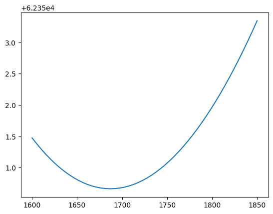
A simple profile#
There is no default function (yet) for simple profiling plot. However, again, we’re in Python and it’s simple enough to do that for a parameter. Let’s do it for sig_yield
x = np.linspace(1600, 1850, num=50)
y = []
sig_yield.floating = False
tmpres = None
for val in tqdm.tqdm(x):
    sig_yield.set_value(val)
    tmpres = minimizer.minimize(nll, init=tmpres)
    y.append(nll.value())

sig_yield.floating = True
result.update_params();  # reset params, equivalent to below
# zfit.param.set_values(nll.get_params(), result)
plt.plot(x, y)
[<matplotlib.lines.Line2D at 0x71949478f440>]
We can also access the covariance matrix of the parameters
result.covariance()
array([[ 4.75994523e+03,  8.83152818e+02, -3.95748195e+03,
        -1.76941694e+01,  4.21964110e+01],
       [ 8.83152818e+02,  3.29096607e+03, -3.54390218e+03,
        -4.78275938e+00,  1.20438809e+01],
       [-3.95748195e+03, -3.54390218e+03,  1.51865146e+04,
         2.24791874e+01, -5.42473287e+01],
       [-1.76941694e+01, -4.78275938e+00,  2.24791874e+01,
         1.82425247e+00, -3.06369272e-01],
       [ 4.21964110e+01,  1.20438809e+01, -5.42473287e+01,
        -3.06369272e-01,  1.64592297e+00]])
Saving and loading#
A FitResult can be saved to disk and loaded back, as can be any other zfit object. This is done using dill, which is like pickle, a Python standard library to serialize arbitrary Python objects.
This allows not only to store single objects but any combination of them. It is recommended therfore to store a dict, or anything arbitrary, with all the objects that are required to reproduce the result.
(the FitResult itself stores all objects too, so it is usually enough to store the FitResult itself)
Make sure to dumb and load all required objects at once. Otherwise, there will be issues regarding parameter names, as it is not clear whether the same or a different object is meant.
dumped_res = zfit.dill.dumps(result)
dumbed_ws = zfit.dill.dumps({'result': result, 'model': model_ext_sum, 'cov': result.covariance(), # usually not needed, as result contains all information
                             'other': ['any', 'other', 'object', mu], 'profile': y})
loaded_res = zfit.dill.loads(dumped_res)
You can try to dump and load losses or PDFs in a HS\(^3\)-like format, a human-readable serialization format. This is however not recommended for long-term storage, as the format may change and is not guaranteed to be stable. (but great for publishing the likelihood!)
zfit.hs3.dumps(nll)
{'metadata': {'HS3': {'version': 'experimental'},
  'serializer': {'lib': 'zfit', 'version': '0.28.0'}},
 'distributions': {'SumPDF': {'type': 'SumPDF',
   'name': 'SumPDF',
   'pdfs': [{'type': 'Gauss',
     'extended': 'sig_yield',
     'name': 'Gauss',
     'x': {'type': 'Space',
      'name': 'mass',
      'min': np.float64(0.0),
      'max': np.float64(1000.0)},
     'mu': 'mu_sig',
     'sigma': 'sigma_sig'},
    {'type': 'Exponential',
     'extended': 'comb_bkg_yield',
     'name': 'Exponential_ext',
     'x': {'type': 'Space',
      'name': 'mass',
      'min': np.float64(0.0),
      'max': np.float64(1000.0)},
     'lam': 'lambda'},
    {'type': 'KDE1DimFFT',
     'extended': 'part_reco_yield',
     'name': 'KDE1DimFFT',
     'data': {'type': 'Data',
      'data': array([[231.96921965],
             [ 66.6452926 ],
             [238.73208904],
             ...,
             [334.33304515],
             [251.48180109],
             [425.15198868]], shape=(18188, 1)),
      'space': [{'type': 'Space',
        'name': 'mass',
        'min': np.float64(0.0),
        'max': np.float64(1000.0)}]},
     'obs': {'type': 'Space',
      'name': 'mass',
      'min': np.float64(0.0),
      'max': np.float64(1000.0)}}],
   'fracs': ['Composed_autoparam_5',
    'Composed_autoparam_6',
    'Composed_autoparam_7']}},
 'variables': {'Composed_autoparam_4': {'name': 'Composed_autoparam_4',
   'func': '80049520020000000000008c0a64696c6c2e5f64696c6c948c105f6372656174655f66756e6374696f6e9493942868008c0c5f6372656174655f636f64659493942843020201944b014b004b004b014b064a13000001435a9700740100000000000000006a02000000000000000000000000000000000000740500000000000000007c006a07000000000000000000000000000000000000ab00000000000000ab01000000000000ab010000000000005300944e8594288c037a6e70948c0373756d948c046c697374948c0676616c7565739474948c06706172616d739485948c832f686f6d652f646f63732f636865636b6f7574732f72656164746865646f63732e6f72672f757365725f6275696c64732f7a6669742d7475746f7269616c732f656e76732f6c61746573742f6c69622f707974686f6e332e31322f736974652d7061636b616765732f7a6669742f6d6f64656c732f6261736566756e63746f722e7079948c0f73756d5f7969656c64735f66756e63948c2d5f70726570726f636573735f696e69745f73756d2e3c6c6f63616c733e2e73756d5f7969656c64735f66756e63944be7431c8000dc1316973791379c34a006a70da10da30fd31b30d31331d00c3194430094292974945294637a6669742e6d6f64656c732e6261736566756e63746f720a5f5f646963745f5f0a68104e4e749452947d947d94288c0f5f5f616e6e6f746174696f6e735f5f947d948c0c5f5f7175616c6e616d655f5f946811758694622e',
   'params': {'yield_0': 'sig_yield',
    'yield_1': 'comb_bkg_yield',
    'yield_2': 'part_reco_yield'},
   'internal_params': {'yield_0': {'type': 'Parameter',
     'name': 'sig_yield',
     'value': 1686.2070877570127,
     'min': 0.0,
     'max': 10000.0,
     'stepsize': 1.0,
     'floating': True,
     'label': 'sig_yield'},
    'yield_1': {'type': 'Parameter',
     'name': 'comb_bkg_yield',
     'value': 630.6021172088584,
     'min': 0.0,
     'max': 10000.0,
     'stepsize': 1.0,
     'floating': True,
     'label': 'comb_bkg_yield'},
    'yield_2': {'type': 'Parameter',
     'name': 'part_reco_yield',
     'value': 7683.384127580149,
     'min': 0.0,
     'max': 10000.0,
     'stepsize': 1.0,
     'floating': True,
     'label': 'part_reco_yield'}}},
  'sig_yield': {'name': 'sig_yield',
   'value': 1686.2070877570127,
   'min': 0.0,
   'max': 10000.0,
   'stepsize': 1.0,
   'floating': True,
   'label': 'sig_yield'},
  'comb_bkg_yield': {'name': 'comb_bkg_yield',
   'value': 630.6021172088584,
   'min': 0.0,
   'max': 10000.0,
   'stepsize': 1.0,
   'floating': True,
   'label': 'comb_bkg_yield'},
  'part_reco_yield': {'name': 'part_reco_yield',
   'value': 7683.384127580149,
   'min': 0.0,
   'max': 10000.0,
   'stepsize': 1.0,
   'floating': True,
   'label': 'part_reco_yield'},
  'Composed_autoparam_5': {'name': 'Composed_autoparam_5',
   'func': '800495bc010000000000008c0a64696c6c2e5f64696c6c948c105f6372656174655f66756e6374696f6e9493942868008c0c5f6372656174655f636f6465949394284300944b014b004b004b014b034a13000001431897007c006401190000007c006402190000007a0b00005300944e8c067969656c645f948c0a73756d5f7969656c6473948794298c06706172616d739485948c832f686f6d652f646f63732f636865636b6f7574732f72656164746865646f63732e6f72672f757365725f6275696c64732f7a6669742d7475746f7269616c732f656e76732f6c61746573742f6c69622f707974686f6e332e31322f736974652d7061636b616765732f7a6669742f6d6f64656c732f6261736566756e63746f722e7079948c083c6c616d6264613e948c265f70726570726f636573735f696e69745f73756d2e3c6c6f63616c733e2e3c6c616d6264613e944bed431380009876a068d11f2fb026b81cd13246d21f46946805292974945294637a6669742e6d6f64656c732e6261736566756e63746f720a5f5f646963745f5f0a680d4e4e749452947d947d94288c0f5f5f616e6e6f746174696f6e735f5f947d948c0c5f5f7175616c6e616d655f5f94680e758694622e',
   'params': {'sum_yields': {'type': 'ComposedParameter',
     'name': 'Composed_autoparam_4',
     'func': '80049520020000000000008c0a64696c6c2e5f64696c6c948c105f6372656174655f66756e6374696f6e9493942868008c0c5f6372656174655f636f64659493942843020201944b014b004b004b014b064a13000001435a9700740100000000000000006a02000000000000000000000000000000000000740500000000000000007c006a07000000000000000000000000000000000000ab00000000000000ab01000000000000ab010000000000005300944e8594288c037a6e70948c0373756d948c046c697374948c0676616c7565739474948c06706172616d739485948c832f686f6d652f646f63732f636865636b6f7574732f72656164746865646f63732e6f72672f757365725f6275696c64732f7a6669742d7475746f7269616c732f656e76732f6c61746573742f6c69622f707974686f6e332e31322f736974652d7061636b616765732f7a6669742f6d6f64656c732f6261736566756e63746f722e7079948c0f73756d5f7969656c64735f66756e63948c2d5f70726570726f636573735f696e69745f73756d2e3c6c6f63616c733e2e73756d5f7969656c64735f66756e63944be7431c8000dc1316973791379c34a006a70da10da30fd31b30d31331d00c3194430094292974945294637a6669742e6d6f64656c732e6261736566756e63746f720a5f5f646963745f5f0a68104e4e749452947d947d94288c0f5f5f616e6e6f746174696f6e735f5f947d948c0c5f5f7175616c6e616d655f5f946811758694622e',
     'params': {'yield_0': 'sig_yield',
      'yield_1': 'comb_bkg_yield',
      'yield_2': 'part_reco_yield'},
     'internal_params': {'yield_0': 'sig_yield',
      'yield_1': 'comb_bkg_yield',
      'yield_2': 'part_reco_yield'}},
    'yield_': 'sig_yield'},
   'internal_params': {'sum_yields': {'type': 'ComposedParameter',
     'name': 'Composed_autoparam_4',
     'func': '80049520020000000000008c0a64696c6c2e5f64696c6c948c105f6372656174655f66756e6374696f6e9493942868008c0c5f6372656174655f636f64659493942843020201944b014b004b004b014b064a13000001435a9700740100000000000000006a02000000000000000000000000000000000000740500000000000000007c006a07000000000000000000000000000000000000ab00000000000000ab01000000000000ab010000000000005300944e8594288c037a6e70948c0373756d948c046c697374948c0676616c7565739474948c06706172616d739485948c832f686f6d652f646f63732f636865636b6f7574732f72656164746865646f63732e6f72672f757365725f6275696c64732f7a6669742d7475746f7269616c732f656e76732f6c61746573742f6c69622f707974686f6e332e31322f736974652d7061636b616765732f7a6669742f6d6f64656c732f6261736566756e63746f722e7079948c0f73756d5f7969656c64735f66756e63948c2d5f70726570726f636573735f696e69745f73756d2e3c6c6f63616c733e2e73756d5f7969656c64735f66756e63944be7431c8000dc1316973791379c34a006a70da10da30fd31b30d31331d00c3194430094292974945294637a6669742e6d6f64656c732e6261736566756e63746f720a5f5f646963745f5f0a68104e4e749452947d947d94288c0f5f5f616e6e6f746174696f6e735f5f947d948c0c5f5f7175616c6e616d655f5f946811758694622e',
     'params': {'yield_0': {'type': 'Parameter',
       'name': 'sig_yield',
       'value': 1686.2070877570127,
       'min': 0.0,
       'max': 10000.0,
       'stepsize': 1.0,
       'floating': True,
       'label': 'sig_yield'},
      'yield_1': {'type': 'Parameter',
       'name': 'comb_bkg_yield',
       'value': 630.6021172088584,
       'min': 0.0,
       'max': 10000.0,
       'stepsize': 1.0,
       'floating': True,
       'label': 'comb_bkg_yield'},
      'yield_2': {'type': 'Parameter',
       'name': 'part_reco_yield',
       'value': 7683.384127580149,
       'min': 0.0,
       'max': 10000.0,
       'stepsize': 1.0,
       'floating': True,
       'label': 'part_reco_yield'}},
     'internal_params': {'yield_0': {'type': 'Parameter',
       'name': 'sig_yield',
       'value': 1686.2070877570127,
       'min': 0.0,
       'max': 10000.0,
       'stepsize': 1.0,
       'floating': True,
       'label': 'sig_yield'},
      'yield_1': {'type': 'Parameter',
       'name': 'comb_bkg_yield',
       'value': 630.6021172088584,
       'min': 0.0,
       'max': 10000.0,
       'stepsize': 1.0,
       'floating': True,
       'label': 'comb_bkg_yield'},
      'yield_2': {'type': 'Parameter',
       'name': 'part_reco_yield',
       'value': 7683.384127580149,
       'min': 0.0,
       'max': 10000.0,
       'stepsize': 1.0,
       'floating': True,
       'label': 'part_reco_yield'}}},
    'yield_': {'type': 'Parameter',
     'name': 'sig_yield',
     'value': 1686.2070877570127,
     'min': 0.0,
     'max': 10000.0,
     'stepsize': 1.0,
     'floating': True,
     'label': 'sig_yield'}}},
  'Composed_autoparam_6': {'name': 'Composed_autoparam_6',
   'func': '800495bc010000000000008c0a64696c6c2e5f64696c6c948c105f6372656174655f66756e6374696f6e9493942868008c0c5f6372656174655f636f6465949394284300944b014b004b004b014b034a13000001431897007c006401190000007c006402190000007a0b00005300944e8c067969656c645f948c0a73756d5f7969656c6473948794298c06706172616d739485948c832f686f6d652f646f63732f636865636b6f7574732f72656164746865646f63732e6f72672f757365725f6275696c64732f7a6669742d7475746f7269616c732f656e76732f6c61746573742f6c69622f707974686f6e332e31322f736974652d7061636b616765732f7a6669742f6d6f64656c732f6261736566756e63746f722e7079948c083c6c616d6264613e948c265f70726570726f636573735f696e69745f73756d2e3c6c6f63616c733e2e3c6c616d6264613e944bed431380009876a068d11f2fb026b81cd13246d21f46946805292974945294637a6669742e6d6f64656c732e6261736566756e63746f720a5f5f646963745f5f0a680d4e4e749452947d947d94288c0f5f5f616e6e6f746174696f6e735f5f947d948c0c5f5f7175616c6e616d655f5f94680e758694622e',
   'params': {'sum_yields': {'type': 'ComposedParameter',
     'name': 'Composed_autoparam_4',
     'func': '80049520020000000000008c0a64696c6c2e5f64696c6c948c105f6372656174655f66756e6374696f6e9493942868008c0c5f6372656174655f636f64659493942843020201944b014b004b004b014b064a13000001435a9700740100000000000000006a02000000000000000000000000000000000000740500000000000000007c006a07000000000000000000000000000000000000ab00000000000000ab01000000000000ab010000000000005300944e8594288c037a6e70948c0373756d948c046c697374948c0676616c7565739474948c06706172616d739485948c832f686f6d652f646f63732f636865636b6f7574732f72656164746865646f63732e6f72672f757365725f6275696c64732f7a6669742d7475746f7269616c732f656e76732f6c61746573742f6c69622f707974686f6e332e31322f736974652d7061636b616765732f7a6669742f6d6f64656c732f6261736566756e63746f722e7079948c0f73756d5f7969656c64735f66756e63948c2d5f70726570726f636573735f696e69745f73756d2e3c6c6f63616c733e2e73756d5f7969656c64735f66756e63944be7431c8000dc1316973791379c34a006a70da10da30fd31b30d31331d00c3194430094292974945294637a6669742e6d6f64656c732e6261736566756e63746f720a5f5f646963745f5f0a68104e4e749452947d947d94288c0f5f5f616e6e6f746174696f6e735f5f947d948c0c5f5f7175616c6e616d655f5f946811758694622e',
     'params': {'yield_0': 'sig_yield',
      'yield_1': 'comb_bkg_yield',
      'yield_2': 'part_reco_yield'},
     'internal_params': {'yield_0': 'sig_yield',
      'yield_1': 'comb_bkg_yield',
      'yield_2': 'part_reco_yield'}},
    'yield_': 'comb_bkg_yield'},
   'internal_params': {'sum_yields': {'type': 'ComposedParameter',
     'name': 'Composed_autoparam_4',
     'func': '80049520020000000000008c0a64696c6c2e5f64696c6c948c105f6372656174655f66756e6374696f6e9493942868008c0c5f6372656174655f636f64659493942843020201944b014b004b004b014b064a13000001435a9700740100000000000000006a02000000000000000000000000000000000000740500000000000000007c006a07000000000000000000000000000000000000ab00000000000000ab01000000000000ab010000000000005300944e8594288c037a6e70948c0373756d948c046c697374948c0676616c7565739474948c06706172616d739485948c832f686f6d652f646f63732f636865636b6f7574732f72656164746865646f63732e6f72672f757365725f6275696c64732f7a6669742d7475746f7269616c732f656e76732f6c61746573742f6c69622f707974686f6e332e31322f736974652d7061636b616765732f7a6669742f6d6f64656c732f6261736566756e63746f722e7079948c0f73756d5f7969656c64735f66756e63948c2d5f70726570726f636573735f696e69745f73756d2e3c6c6f63616c733e2e73756d5f7969656c64735f66756e63944be7431c8000dc1316973791379c34a006a70da10da30fd31b30d31331d00c3194430094292974945294637a6669742e6d6f64656c732e6261736566756e63746f720a5f5f646963745f5f0a68104e4e749452947d947d94288c0f5f5f616e6e6f746174696f6e735f5f947d948c0c5f5f7175616c6e616d655f5f946811758694622e',
     'params': {'yield_0': {'type': 'Parameter',
       'name': 'sig_yield',
       'value': 1686.2070877570127,
       'min': 0.0,
       'max': 10000.0,
       'stepsize': 1.0,
       'floating': True,
       'label': 'sig_yield'},
      'yield_1': {'type': 'Parameter',
       'name': 'comb_bkg_yield',
       'value': 630.6021172088584,
       'min': 0.0,
       'max': 10000.0,
       'stepsize': 1.0,
       'floating': True,
       'label': 'comb_bkg_yield'},
      'yield_2': {'type': 'Parameter',
       'name': 'part_reco_yield',
       'value': 7683.384127580149,
       'min': 0.0,
       'max': 10000.0,
       'stepsize': 1.0,
       'floating': True,
       'label': 'part_reco_yield'}},
     'internal_params': {'yield_0': {'type': 'Parameter',
       'name': 'sig_yield',
       'value': 1686.2070877570127,
       'min': 0.0,
       'max': 10000.0,
       'stepsize': 1.0,
       'floating': True,
       'label': 'sig_yield'},
      'yield_1': {'type': 'Parameter',
       'name': 'comb_bkg_yield',
       'value': 630.6021172088584,
       'min': 0.0,
       'max': 10000.0,
       'stepsize': 1.0,
       'floating': True,
       'label': 'comb_bkg_yield'},
      'yield_2': {'type': 'Parameter',
       'name': 'part_reco_yield',
       'value': 7683.384127580149,
       'min': 0.0,
       'max': 10000.0,
       'stepsize': 1.0,
       'floating': True,
       'label': 'part_reco_yield'}}},
    'yield_': {'type': 'Parameter',
     'name': 'comb_bkg_yield',
     'value': 630.6021172088584,
     'min': 0.0,
     'max': 10000.0,
     'stepsize': 1.0,
     'floating': True,
     'label': 'comb_bkg_yield'}}},
  'Composed_autoparam_7': {'name': 'Composed_autoparam_7',
   'func': '800495bc010000000000008c0a64696c6c2e5f64696c6c948c105f6372656174655f66756e6374696f6e9493942868008c0c5f6372656174655f636f6465949394284300944b014b004b004b014b034a13000001431897007c006401190000007c006402190000007a0b00005300944e8c067969656c645f948c0a73756d5f7969656c6473948794298c06706172616d739485948c832f686f6d652f646f63732f636865636b6f7574732f72656164746865646f63732e6f72672f757365725f6275696c64732f7a6669742d7475746f7269616c732f656e76732f6c61746573742f6c69622f707974686f6e332e31322f736974652d7061636b616765732f7a6669742f6d6f64656c732f6261736566756e63746f722e7079948c083c6c616d6264613e948c265f70726570726f636573735f696e69745f73756d2e3c6c6f63616c733e2e3c6c616d6264613e944bed431380009876a068d11f2fb026b81cd13246d21f46946805292974945294637a6669742e6d6f64656c732e6261736566756e63746f720a5f5f646963745f5f0a680d4e4e749452947d947d94288c0f5f5f616e6e6f746174696f6e735f5f947d948c0c5f5f7175616c6e616d655f5f94680e758694622e',
   'params': {'sum_yields': {'type': 'ComposedParameter',
     'name': 'Composed_autoparam_4',
     'func': '80049520020000000000008c0a64696c6c2e5f64696c6c948c105f6372656174655f66756e6374696f6e9493942868008c0c5f6372656174655f636f64659493942843020201944b014b004b004b014b064a13000001435a9700740100000000000000006a02000000000000000000000000000000000000740500000000000000007c006a07000000000000000000000000000000000000ab00000000000000ab01000000000000ab010000000000005300944e8594288c037a6e70948c0373756d948c046c697374948c0676616c7565739474948c06706172616d739485948c832f686f6d652f646f63732f636865636b6f7574732f72656164746865646f63732e6f72672f757365725f6275696c64732f7a6669742d7475746f7269616c732f656e76732f6c61746573742f6c69622f707974686f6e332e31322f736974652d7061636b616765732f7a6669742f6d6f64656c732f6261736566756e63746f722e7079948c0f73756d5f7969656c64735f66756e63948c2d5f70726570726f636573735f696e69745f73756d2e3c6c6f63616c733e2e73756d5f7969656c64735f66756e63944be7431c8000dc1316973791379c34a006a70da10da30fd31b30d31331d00c3194430094292974945294637a6669742e6d6f64656c732e6261736566756e63746f720a5f5f646963745f5f0a68104e4e749452947d947d94288c0f5f5f616e6e6f746174696f6e735f5f947d948c0c5f5f7175616c6e616d655f5f946811758694622e',
     'params': {'yield_0': 'sig_yield',
      'yield_1': 'comb_bkg_yield',
      'yield_2': 'part_reco_yield'},
     'internal_params': {'yield_0': 'sig_yield',
      'yield_1': 'comb_bkg_yield',
      'yield_2': 'part_reco_yield'}},
    'yield_': 'part_reco_yield'},
   'internal_params': {'sum_yields': {'type': 'ComposedParameter',
     'name': 'Composed_autoparam_4',
     'func': '80049520020000000000008c0a64696c6c2e5f64696c6c948c105f6372656174655f66756e6374696f6e9493942868008c0c5f6372656174655f636f64659493942843020201944b014b004b004b014b064a13000001435a9700740100000000000000006a02000000000000000000000000000000000000740500000000000000007c006a07000000000000000000000000000000000000ab00000000000000ab01000000000000ab010000000000005300944e8594288c037a6e70948c0373756d948c046c697374948c0676616c7565739474948c06706172616d739485948c832f686f6d652f646f63732f636865636b6f7574732f72656164746865646f63732e6f72672f757365725f6275696c64732f7a6669742d7475746f7269616c732f656e76732f6c61746573742f6c69622f707974686f6e332e31322f736974652d7061636b616765732f7a6669742f6d6f64656c732f6261736566756e63746f722e7079948c0f73756d5f7969656c64735f66756e63948c2d5f70726570726f636573735f696e69745f73756d2e3c6c6f63616c733e2e73756d5f7969656c64735f66756e63944be7431c8000dc1316973791379c34a006a70da10da30fd31b30d31331d00c3194430094292974945294637a6669742e6d6f64656c732e6261736566756e63746f720a5f5f646963745f5f0a68104e4e749452947d947d94288c0f5f5f616e6e6f746174696f6e735f5f947d948c0c5f5f7175616c6e616d655f5f946811758694622e',
     'params': {'yield_0': {'type': 'Parameter',
       'name': 'sig_yield',
       'value': 1686.2070877570127,
       'min': 0.0,
       'max': 10000.0,
       'stepsize': 1.0,
       'floating': True,
       'label': 'sig_yield'},
      'yield_1': {'type': 'Parameter',
       'name': 'comb_bkg_yield',
       'value': 630.6021172088584,
       'min': 0.0,
       'max': 10000.0,
       'stepsize': 1.0,
       'floating': True,
       'label': 'comb_bkg_yield'},
      'yield_2': {'type': 'Parameter',
       'name': 'part_reco_yield',
       'value': 7683.384127580149,
       'min': 0.0,
       'max': 10000.0,
       'stepsize': 1.0,
       'floating': True,
       'label': 'part_reco_yield'}},
     'internal_params': {'yield_0': {'type': 'Parameter',
       'name': 'sig_yield',
       'value': 1686.2070877570127,
       'min': 0.0,
       'max': 10000.0,
       'stepsize': 1.0,
       'floating': True,
       'label': 'sig_yield'},
      'yield_1': {'type': 'Parameter',
       'name': 'comb_bkg_yield',
       'value': 630.6021172088584,
       'min': 0.0,
       'max': 10000.0,
       'stepsize': 1.0,
       'floating': True,
       'label': 'comb_bkg_yield'},
      'yield_2': {'type': 'Parameter',
       'name': 'part_reco_yield',
       'value': 7683.384127580149,
       'min': 0.0,
       'max': 10000.0,
       'stepsize': 1.0,
       'floating': True,
       'label': 'part_reco_yield'}}},
    'yield_': {'type': 'Parameter',
     'name': 'part_reco_yield',
     'value': 7683.384127580149,
     'min': 0.0,
     'max': 10000.0,
     'stepsize': 1.0,
     'floating': True,
     'label': 'part_reco_yield'}}},
  'mu_sig': {'name': 'mu_sig',
   'value': 369.51971503868464,
   'min': 100.0,
   'max': 600.0,
   'stepsize': 0.01,
   'floating': True,
   'label': 'mu_sig'},
  'sigma_sig': {'name': 'sigma_sig',
   'value': 31.85403816876303,
   'min': 1.0,
   'max': 100.0,
   'stepsize': 0.01,
   'floating': True,
   'label': 'sigma_sig'},
  'lambda': {'name': 'lambda',
   'value': -0.013913462388517801,
   'min': -0.05,
   'max': -1e-05,
   'stepsize': 0.01,
   'floating': False,
   'label': 'lambda'},
  'FIXED_autoparam_3': {'name': 'FIXED_autoparam_3',
   'value': 16.173146438297277,
   'floating': False,
   'label': 'FIXED_autoparam_3'},
  'mass': {'name': 'mass', 'min': np.float64(0.0), 'max': np.float64(1000.0)}},
 'loss': {'ExtendedUnbinnedNLL': {'type': 'ExtendedUnbinnedNLL',
   'model': [{'type': 'SumPDF',
     'name': 'SumPDF',
     'pdfs': [{'type': 'Gauss',
       'extended': 'sig_yield',
       'name': 'Gauss',
       'x': {'type': 'Space',
        'name': 'mass',
        'min': np.float64(0.0),
        'max': np.float64(1000.0)},
       'mu': 'mu_sig',
       'sigma': 'sigma_sig'},
      {'type': 'Exponential',
       'extended': 'comb_bkg_yield',
       'name': 'Exponential_ext',
       'x': {'type': 'Space',
        'name': 'mass',
        'min': np.float64(0.0),
        'max': np.float64(1000.0)},
       'lam': 'lambda'},
      {'type': 'KDE1DimFFT',
       'extended': 'part_reco_yield',
       'name': 'KDE1DimFFT',
       'data': {'type': 'Data',
        'data': array([[231.96921965],
               [ 66.6452926 ],
               [238.73208904],
               ...,
               [334.33304515],
               [251.48180109],
               [425.15198868]], shape=(18188, 1)),
        'space': [{'type': 'Space',
          'name': 'mass',
          'min': np.float64(0.0),
          'max': np.float64(1000.0)}]},
       'obs': {'type': 'Space',
        'name': 'mass',
        'min': np.float64(0.0),
        'max': np.float64(1000.0)}}],
     'fracs': ['Composed_autoparam_5',
      'Composed_autoparam_6',
      'Composed_autoparam_7']}],
   'data': [{'type': 'Data',
     'data': array([[168.55305948],
            [318.58112707],
            [238.48427593],
            ...,
            [371.76005469],
            [208.36938779],
            [151.65755148]], shape=(10000, 1)),
     'space': [{'type': 'Space',
       'name': 'mass',
       'min': np.float64(0.0),
       'max': np.float64(1000.0)}]}],
   'constraints': [],
   'options': {}}},
 'data': {None: {'type': 'Data',
   'data': array([[168.55305948],
          [318.58112707],
          [238.48427593],
          ...,
          [371.76005469],
          [208.36938779],
          [151.65755148]], shape=(10000, 1)),
   'space': [{'type': 'Space',
     'name': 'mass',
     'min': np.float64(0.0),
     'max': np.float64(1000.0)}]}},
 'constraints': {}}
# or just a PDF/parts of it
signal.to_yaml()
'\'{"type": "CrystalBall", "name": "CrystalBall", "x": {"type": "Space", "name": "mass",\n "min": 0.0, "max": 1000.0}, "mu": {"type": "Parameter", "name": "mu_sig", "value":\n 369.51971503868464, "min": 100.0, "max": 600.0, "stepsize": 0.01, "floating": true,\n "label": "mu_sig"}, "sigma": {"type": "Parameter", "name": "sigma_sig", "value":\n 31.85403816876303, "min": 1.0, "max": 100.0, "stepsize": 0.01, "floating": true,\n "label": "sigma_sig"}, "alpha": {"type": "Parameter", "name": "alpha_sig", "value":\n 200.0, "min": 100.0, "max": 400.0, "stepsize": 0.01, "floating": false, "label":\n "alpha_sig"}, "n": {"type": "Parameter", "name": "n sig", "value": 4.0, "min": 0.1,\n "max": 30.0, "stepsize": 0.01, "floating": false, "label": "n sig"}}\'\n'
End of zfit - Extended#
This is where zfit finishes and other libraries take over.
Beginning of hepstats - Extended#
hepstats is a library containing statistical tools and utilities for high energy physics. In particular you do statistical inferences using the models and likelhoods function constructed in zfit.
Short example: let’s compute for instance a confidence interval at 68 % confidence level on the mean of the gaussian defined above.
from hepstats.hypotests import ConfidenceInterval
from hepstats.hypotests.calculators import AsymptoticCalculator
from hepstats.hypotests.parameters import POIarray
calculator = AsymptoticCalculator(input=result, minimizer=minimizer)
value = result.params[mu_sig]["value"]
error = result.params[mu_sig]["hesse"]["error"]

mean_scan = POIarray(mu_sig, np.linspace(value - 1.5 * error, value + 1.5 * error, 10))
ci = ConfidenceInterval(calculator, mean_scan)
# ci.interval() # fix in hepstats
# from utils import one_minus_cl_plot

# ax = one_minus_cl_plot(ci)
# ax.set_xlabel("mean")
There will be more of hepstats later.