Quickstart

In this quick tutorial, we’ll show the basic ideas on what you can do with zfit, without going into much detail or performing advanced tasks.

import matplotlib.pyplot as plt
import mplhep
import numpy as np
import zfit
import zfit.z.numpy as znp  # numpy-like backend

Create observables

The observable space in which PDFs are defined is created with the Space class

obs = zfit.Space('x', -10, 10)

Create data

We create some unbinned data using numpy. Other constructors, e.g. for ROOT files are also available.

mu_true = 0
sigma_true = 1

data_np = np.random.normal(mu_true, sigma_true, size=10000)
data = zfit.Data(data=data_np, obs=obs)

Create a PDF to fit

Let’s create a Gaussian PDF so we can fit the dataset. To do this, first we create the fit parameters, which follow a convention similar to RooFit:

zfit.Parameter(name, initial_value, lower_limit (optional), upper_limit (optional), other options)

mu = zfit.Parameter("mu", 2.4, -1., 5., step_size=0.001)  # step_size is not mandatory but can be helpful
sigma = zfit.Parameter("sigma", 1.3, 0, 5., step_size=0.001)  # it should be around the estimated uncertainty

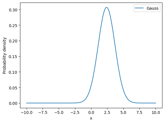
Now we instantiate a Gaussian from the zfit PDF library (more on how to create your own PDFs later)

gauss = zfit.pdf.Gauss(obs=obs, mu=mu, sigma=sigma)

gauss.plot.plotpdf()

<Axes: xlabel='x', ylabel='Probability density'>

This pdf contains several useful methods, such as calculating a probability, calculating its integral, sampling etc.

# Let's get some probabilities.
consts = [-1, 0, 1]
probs = gauss.pdf(consts)
print(f"x values: {consts}\nresult:   {probs}")

x values: [-1, 0, 1]
result:   [0.01003756 0.05582995 0.17184121]

Fitting

To fit, we need to take three steps: create the negative \(\log\mathcal{L}\), instantiate a minimizer and then minimize the likelihood.

# Create the negative log likelihood

nll = zfit.loss.UnbinnedNLL(model=gauss, data=data)  # loss

# Load and instantiate a minimizer
minimizer = zfit.minimize.Minuit()
result = minimizer.minimize(loss=nll)

print(result)

FitResult

 of
<UnbinnedNLL model=[<zfit.<class 'zfit.models.dist_tfp.Gauss'>  params=[mu, sigma]] data=[<zfit.Data: Data obs=('x',) shape=(10000, 1)>] constraints=[]> 
with
<Minuit Minuit, tol=0.001>

╒═════════╤═════════════╤══════════════════╤═════════╤══════════════════════════════╕
│  valid  │  converged  │  param at limit  │   edm   │   approx. fmin (full | opt.) │
╞═════════╪═════════════╪══════════════════╪═════════╪══════════════════════════════╡
│  

True

   │    True

     │      False

       │ 2.5e-05 │         14214.59 | -7816.398 │
╘═════════╧═════════════╧══════════════════╧═════════╧══════════════════════════════╛

Parameters

name      value  (rounded)    at limit
------  ------------------  ----------
mu              -0.0142918       False

sigma              1.00257       False

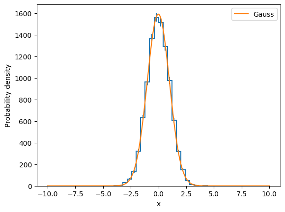
And we can plot the result to see how it went.

%matplotlib inline

n_bins = 50
mplhep.histplot(data.to_binned(50))
rescale = obs.v1.volume / n_bins * float(data.nevents)
ax = gauss.plot.plotpdf(scale=rescale)

# x = np.linspace(*obs.v1.limits, num=1000)
# probs = gauss.pdf(x)
# _ = plt.plot(x, rescale * probs)

obs.v1.volume

<tf.Tensor: shape=(1,), dtype=float64, numpy=array([20.])>

The FitResult that we obtained contains information about the minimization and can now be used to calculate the errors

print(f"Function result: {result.fmin}", result.fmin)
print(f"Converged: {result.converged} and valid: {result.valid}", )
print(result)

Function result: 14214.594513283286

14214.594513283286

Converged: True and valid: True

FitResult

 of
<UnbinnedNLL model=[<zfit.<class 'zfit.models.dist_tfp.Gauss'>  params=[mu, sigma]] data=[<zfit.Data: Data obs=('x',) shape=(10000, 1)>] constraints=[]> 
with
<Minuit Minuit, tol=0.001>

╒═════════╤═════════════╤══════════════════╤═════════╤══════════════════════════════╕
│  valid  │  converged  │  param at limit  │   edm   │   approx. fmin (full | opt.) │
╞═════════╪═════════════╪══════════════════╪═════════╪══════════════════════════════╡
│  

True

   │    True

     │      False

       │ 2.5e-05 │         14214.59 | -7816.398 │
╘═════════╧═════════════╧══════════════════╧═════════╧══════════════════════════════╛

Parameters

name      value  (rounded)    at limit
------  ------------------  ----------
mu              -0.0142918       False

sigma              1.00257       False

# we still have access to everything
result.loss.model[0]

<zfit.<class 'zfit.models.dist_tfp.Gauss'>  params=[mu, sigma]

hesse_errors = result.hesse()
minos_errors = result.errors()

print(result)

FitResult

 of
<UnbinnedNLL model=[<zfit.<class 'zfit.models.dist_tfp.Gauss'>  params=[mu, sigma]] data=[<zfit.Data: Data obs=('x',) shape=(10000, 1)>] constraints=[]> 
with
<Minuit Minuit, tol=0.001>

╒═════════╤═════════════╤══════════════════╤═════════╤══════════════════════════════╕
│  valid  │  converged  │  param at limit  │   edm   │   approx. fmin (full | opt.) │
╞═════════╪═════════════╪══════════════════╪═════════╪══════════════════════════════╡
│  

True

   │    True

     │      False

       │ 2.5e-05 │         14214.59 | -7816.398 │
╘═════════╧═════════════╧══════════════════╧═════════╧══════════════════════════════╛

Parameters

name      value  (rounded)        hesse               errors    at limit
------  ------------------  -----------  -------------------  ----------
mu              -0.0142918  +/-    0.01  -   0.01   +   0.01       False

sigma              1.00257  +/-  0.0071  - 0.0071   + 0.0071       False

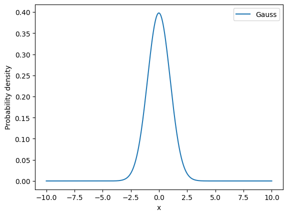
Storing the result

Everything is accessible, feel free to store it in your own format

dumped = zfit.dill.dumps(result)  # like pickle
loaded = zfit.dill.loads(dumped)
loadedpdf = loaded.loss.model[0]
loadedpdf.plot.plotpdf()

<Axes: xlabel='x', ylabel='Probability density'>

zfit.hs3.dumps(nll)  # experimental, human-readable serialization

{'metadata': {'HS3': {'version': 'experimental'},
  'serializer': {'lib': 'zfit', 'version': '0.28.0'}},
 'distributions': {'Gauss': {'type': 'Gauss',
   'name': 'Gauss',
   'x': {'type': 'Space',
    'name': 'x',
    'min': np.float64(-10.0),
    'max': np.float64(10.0)},
   'mu': 'mu',
   'sigma': 'sigma'}},
 'variables': {'mu': {'name': 'mu',
   'value': -0.014291760485314078,
   'min': -1.0,
   'max': 5.0,
   'stepsize': 0.001,
   'floating': True,
   'label': 'mu'},
  'sigma': {'name': 'sigma',
   'value': 1.0025665286080736,
   'min': 0.0,
   'max': 5.0,
   'stepsize': 0.001,
   'floating': True,
   'label': 'sigma'},
  'x': {'name': 'x', 'min': np.float64(-10.0), 'max': np.float64(10.0)}},
 'loss': {'UnbinnedNLL': {'type': 'UnbinnedNLL',
   'model': [{'type': 'Gauss',
     'name': 'Gauss',
     'x': {'type': 'Space',
      'name': 'x',
      'min': np.float64(-10.0),
      'max': np.float64(10.0)},
     'mu': 'mu',
     'sigma': 'sigma'}],
   'data': [{'type': 'Data',
     'data': array([[ 0.48494449],
            [ 0.19313535],
            [ 1.1827559 ],
            ...,
            [-1.32702267],
            [ 0.60526347],
            [-0.38265208]], shape=(10000, 1)),
     'space': [{'type': 'Space',
       'name': 'x',
       'min': np.float64(-10.0),
       'max': np.float64(10.0)}]}],
   'constraints': [],
   'options': {}}},
 'data': {None: {'type': 'Data',
   'data': array([[ 0.48494449],
          [ 0.19313535],
          [ 1.1827559 ],
          ...,
          [-1.32702267],
          [ 0.60526347],
          [-0.38265208]], shape=(10000, 1)),
   'space': [{'type': 'Space',
     'name': 'x',
     'min': np.float64(-10.0),
     'max': np.float64(10.0)}]}},
 'constraints': {}}