Binned fits

Binned models and data can be created in two ways:

• from an unbinned model to a binned model or an unbinned dataset to a binned dataset

• directly from a binned object

import hist as hist
import mplhep
import numpy as np
import zfit
import zfit.z.numpy as znp

from matplotlib import pyplot as plt

normal_np = np.random.normal(loc=2., scale=3., size=10000)

obs = zfit.Space("x", -10, 10)

mu = zfit.Parameter("mu", 1., -4, 6)
sigma = zfit.Parameter("sigma", 1., 0.1, 10)
model_nobin = zfit.pdf.Gauss(mu, sigma, obs)

data_nobin = zfit.Data.from_numpy(obs, normal_np)

loss_nobin = zfit.loss.UnbinnedNLL(model_nobin, data_nobin)

# make binned
binning = zfit.binned.RegularBinning(50, -8, 10, name="x")
obs_bin = zfit.Space("x", binning=binning)

data = data_nobin.to_binned(obs_bin)
model = model_nobin.to_binned(obs_bin)
loss = zfit.loss.BinnedNLL(model, data)

Minimization

Both loss look the same to a minimizer and from here on, the whole minimization process is the same.

The following is the same as in the most simple case.

minimizer = zfit.minimize.Minuit()
result = minimizer.minimize(loss)

result.hesse()
print(result)

FitResult

 of
<BinnedNLL model=[<zfit.models.tobinned.BinnedFromUnbinnedPDF object at 0x7f4844320690>] data=[<zfit._data.binneddatav1.BinnedData object at 0x7f47d5d0cb50>] constraints=[]> 
with
<Minuit Minuit tol=0.001>

╒═════════╤═════════════╤══════════════════╤════════╤══════════════════════════════╕
│  valid  │  converged  │  param at limit  │  edm   │   approx. fmin (full | opt.) │
╞═════════╪═════════════╪══════════════════╪════════╪══════════════════════════════╡
│  

True

   │    True

     │      False

       │ 0.0005 │        -46660.05 | -46608.87 │
╘═════════╧═════════════╧══════════════════╧════════╧══════════════════════════════╛

Parameters

name      value  (rounded)        hesse    at limit
------  ------------------  -----------  ----------
mu                 1.99472  +/-   0.031       False

sigma              3.02477  +/-   0.023       False

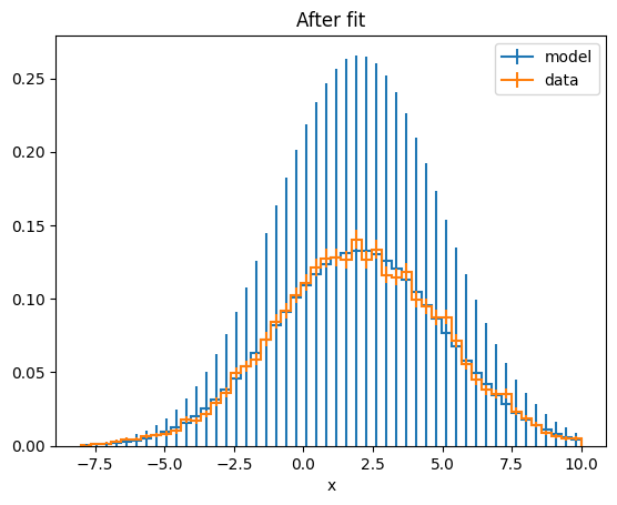
Plotting the PDF

Since both PDFs are histograms, they can both be converted to histograms and plotted.

Using the to_hist method of the model and the BinnedData respectively, the data can be converted to a histogram.

model_hist = model.to_hist()

plt.figure()
mplhep.histplot(model_hist, density=1, label="model")
mplhep.histplot(data, density=1, label="data")
plt.legend()
plt.title("After fit")

Text(0.5, 1.0, 'After fit')

To and from histograms

zfit interoperates with the Scikit-HEP histogram packages hist and boost-histogram, most notably with the NamedHist (or Hist if axes have a name) class.

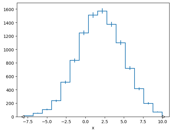
We can create a BinnedData from a (Named)Hist and vice versa.

h = hist.Hist(hist.axis.Regular(bins=15, start=-8, stop=10, name="x"))
h.fill(x=normal_np)
mplhep.histplot(h)

[StairsArtists(stairs=<matplotlib.patches.StepPatch object at 0x7f47b9b02f10>, errorbar=<ErrorbarContainer object of 3 artists>, legend_artist=<ErrorbarContainer object of 3 artists>)]

binned_data = zfit.data.BinnedData.from_hist(h)
binned_data

Regular(15, -8, 10, underflow=False, overflow=False, name='x')

---

Weight() Σ=WeightedSum(value=9965, variance=9965)

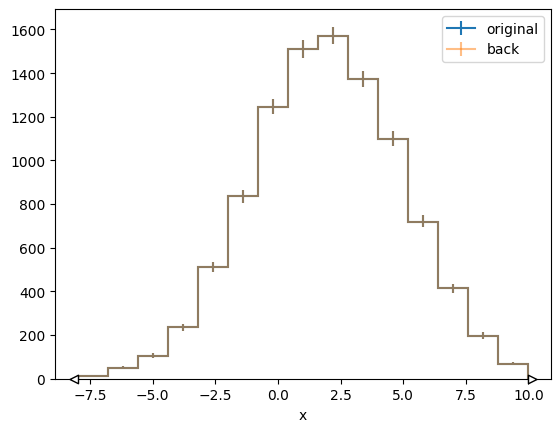
# convert back to hist
h_back = binned_data.to_hist()

plt.figure()
mplhep.histplot(h, label="original")
mplhep.histplot(h_back, label="back", alpha=0.5)
plt.legend()

<matplotlib.legend.Legend at 0x7f47b9a017d0>

Binned models from histograms

With a binned dataset, we can directly create a model from it using HistogramPDF. In fact, we could even directly use the histogram to create a HistogramPDF from it.

histpdf = zfit.pdf.HistogramPDF(h)

As previous models, this is a Binned PDF, so we can:

• use the to_hist method to get a (Named)Hist back.

• use the to_binned method to get a BinnedData back.

• use the counts method to get the counts of the histogram.

• use the rel_counts method to get the relative counts of the histogram.

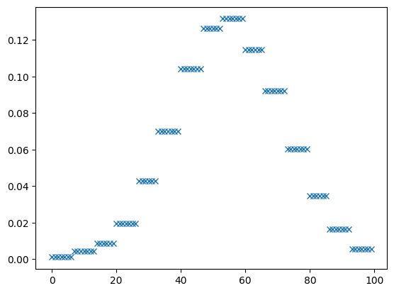
Furthermore, HistogramPDF also has the pdf and ext_pdf method like an unbined PDF. They return a BinnedData if a BinnedData is passed to them (where no evaluation is done on the data passed, just the axes are used). Both methods, pdf and ext_pdf, can also handle unbinned data.

x = znp.linspace(-8, 10, 100)
plt.plot(histpdf.pdf(x), 'x')

[<matplotlib.lines.Line2D at 0x7f47b9adee90>]

We can also go the other way around and produce a Hist from a HistogramPDF. There are two distinct ways to do this:

• using the to_hist or to_binneddata method of the HistogramPDF to create a Hist or a BinnedData respectively that represents the exact shape of the PDF.

• draw a sample from the histogram using the sample method. This will not result in an exact match to the PDFs shape but will have random fluctuations. This functionality can be used for example to perform toy studies.

azimov_hist = model.to_hist()
azimov_data = model.to_binneddata()
sampled_data = model.sample(1000)

# The exact histogram from the PDF
azimov_data

Regular(50, -8, 10, underflow=False, overflow=False, name='x')

---

Weight() Σ=WeightedSum(value=1, variance=nan) (WeightedSum(value=1, variance=nan) with flow)

# A sample from the histogram
sampled_data

Regular(50, -8, 10, underflow=False, overflow=False, name='x')

---

Weight() Σ=WeightedSum(value=1000, variance=nan) (WeightedSum(value=1000, variance=nan) with flow)