Kernel Density Estimation#
This notebook is an introduction into the practical usage of KDEs in zfit and explains the different parameters. A complete introduction to Kernel Density Estimations, explanations to all methods implemented in zfit and a throughout comparison of the performance can be either found in Performance of univariate kernel density estimation methods in TensorFlow by Marc Steiner from which parts here are taken or in the documentation of zfit
Kernel Density Estimation is a non-parametric method to estimate the density of a population and offers a more accurate way than a histogram. In a kernel density estimation each data point is substituted with a kernel function that specifies how much it influences its neighboring regions. This kernel functions can then be summed up to get an estimate of the probability density distribution, quite similarly as summing up data points inside bins.
However, since the kernel functions are centered on the data points directly, KDE circumvents the problem of arbitrary bin positioning. KDE still depends on the kernel bandwidth (a measure of the spread of the kernel function), however, the total PDF does depend less strongly on the kernel bandwidth than histograms do on bin width and it is much easier to specify rules for an approximately optimal kernel bandwidth than it is to do so for bin width.
Definition#
Given a set of \(n\) sample points \(x_k\) (\(k = 1,\cdots,n\)), kernel density estimation \(\widehat{f}_h(x)\) is defined as
where \(K(x)\) is called the kernel function, \(h\) is the bandwidth of the kernel and \(x\) is the value for which the estimate is calculated. The kernel function defines the shape and size of influence of a single data point over the estimation, whereas the bandwidth defines the range of influence. Most typically a simple Gaussian distribution (\(K(x) :=\frac{1}{\sqrt{2\pi}}e^{-\frac{1}{2}x^2}\)) is used as kernel function. The larger the bandwidth parameter \(h\) the larger is the range of influence of a single data point on the estimated distribution.
Weights#
It is straightforward to add event weights in the above expression. zfit KDE fully support weights in data samples and will be taken into account automatically in the KDE.
Computational complexity#
This leads for a large n however to computational problems, as the computational complexity of the exact KDE above is given by \(\mathcal{O}(nm)\) where \(n\) is the number of sample points to estimate from and \(m\) is the number of evaluation points (the points where you want to calculate the estimate).
To circumvent this problem, there exist several approximative methods to decrease this complexity and therefore decrease the runtime as well.
Hint on running the notebook
Feel free to rerun a cell a few times. This will change the sample drawn and gives an impression of how the PDF based on this sample could also look like.
import matplotlib.pyplot as plt
import mplhep
import numpy as np
import zfit

np.random.seed(23)
Exact KDE#
Using the definition above of a KDE, this is implemented in the KDE1DimExact. We can start out with a simple Gaussian.
obs_wide = zfit.Space('x', (-10, 10))
x = np.linspace(-10, 10, 200)
gauss = zfit.pdf.Gauss(obs=obs_wide, mu=0, sigma=2)
sample = gauss.sample(60)
sample_np = zfit.run(sample.value())

kde = zfit.pdf.KDE1DimExact(sample,
                            # obs,
                            # kernel,
                            # padding,
                            # weights,
                            # name
                            )
plt.plot(x, kde.pdf(x), label='Default exact KDE')
plt.plot(x, gauss.pdf(x), label='True PDF')
plt.plot(sample_np, np.zeros_like(sample_np), 'b|', ms=12)
plt.legend()
<matplotlib.legend.Legend at 0x771ac920e060>
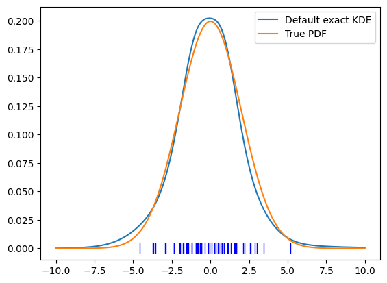
This looks already reasonable and we see that the PDF is overestimated in the regions where we sampled, by chance, many events and underestimated in other regions. Since this was a simple example, /et’s create a more complitated one (and let’s use a bit more samples in order to be able to infer the shape).
gauss1 = zfit.pdf.Gauss(obs=obs_wide, mu=0, sigma=2)
gauss2 = zfit.pdf.Gauss(obs=obs_wide, mu=3, sigma=0.5)
true_pdf = zfit.pdf.SumPDF([gauss1, gauss2], fracs=0.85)
sample = true_pdf.sample(1000)
sample_np = zfit.run(sample.value())

kde = zfit.pdf.KDE1DimExact(sample,
                            # obs,
                            # kernel,
                            # padding,
                            # weights,
                            # name
                            )
plt.plot(x, kde.pdf(x), label='Default exact KDE')
plt.plot(x, true_pdf.pdf(x), label='True PDF')
plt.legend()
<matplotlib.legend.Legend at 0x771ac6d2f410>
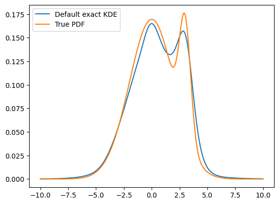
This is more difficult, actually impossible for the current configuration, to approximate the actual PDF well, because we use by default a single bandwidth.
Bandwidth#
The bandwidth of a kernel defines it’s width, corresponding to the sigma of a Gaussian distribution. There is a distinction between global and local bandwidth:
- Global bandwidth
- A is a single parameter that is shared amongst all kernels. While this is a fast and robust method, it is a rule of thumb approximation. Due to its global nature, it cannot take into account the different varying local densities.
- Local bandwidth
- A local bandwidth means that each kernel $i$ has a different bandwidth. In other words, given some data points with size $n$, we will need $n$ bandwidth parameters. This is often more accurate than a global bandwidth, as it allows to have larger bandwiths in areas of smaller density, where, due to the small local sample size, we have less certainty over the true density while having a smaller bandwidth in denser populated areas.
We can compare the effects of different global bandwidths
plt.plot(x, true_pdf.pdf(x), label='True PDF')

for h in [0.1, 0.5, 2, 10]:
    kde = zfit.pdf.KDE1DimExact(sample, bandwidth=h)
    plt.plot(x, kde.pdf(x), '--', alpha=0.6, label=f'KDE h={h}')
plt.legend()
<matplotlib.legend.Legend at 0x771ac6dbf4a0>
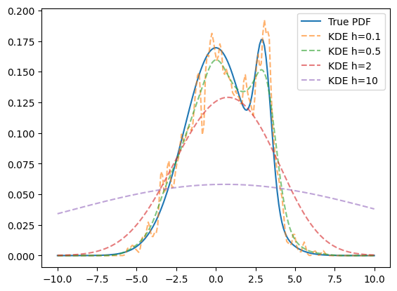
Making the bandwidth larger makes the KDE less dependent on the randomness of the sample and overfitting of it while it tends to smear out features. 0.1 is clearly too wigly while 2 already smears out the feature of having actually two Gaussian peaks.
There are a few methods to estimate the optimal global bandwidth, Silvermans (default) and Scotts rule of thumb, respectively. There are also adaptive methods implemented that create an initial density estimation with a rule of thumb and use it to define local bandwidth that are inversely proportional to the (squareroot of) the density.
kdes_all = [("silverman", '--'), ("scott", '--'), ("adaptive_geom", ':'), ("adaptive_zfit", ':'), ("isj", '-.')]
kdes_some = [("silverman", '--'), ("adaptive_zfit", ':'), ("isj", '-.')]
for subplot in range(1, 4):
    plt.figure(subplot)
    if subplot != 1:
        # let's zoom in to better see the details
        plt.xlim(-2.5, 4)
        plt.ylim(0.1, 0.2)
    plt.plot(x, true_pdf.pdf(x), 'k', label='True PDF')
    kdes = kdes_some if subplot == 3 else kdes_all
    for h, fmt in kdes:
        kde = zfit.pdf.KDE1DimExact(sample, bandwidth=h)
        plt.plot(x, kde.pdf(x), fmt, alpha=0.8, label=f'KDE {h}')
    plt.legend()
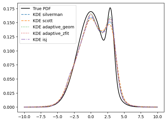
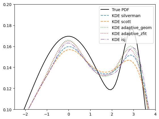
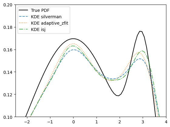
As we can see, the adaptive method and “isj” (we will see more on that later on) better takes into account the nuances of the peaks. It is very well possible to use local bandwidths directly as an array parameter to bandwidth.
Kernel#
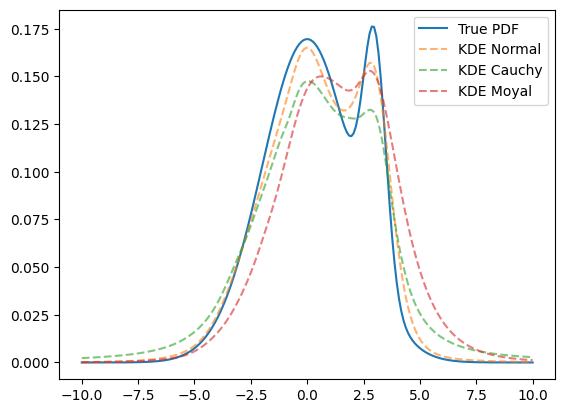
The kernel is the heart of the Kernel Density Estimation, which consists of the sum of kernels around each sample point. Therefore, a kernel should represent the distribution probability of a single data point as close as possible.
The most widespread kernel is a Gaussian, or Normal, distribution as many real world example follow it. However, there are many cases where this assumption is not per-se true. In this cases an alternative kernel may offers a better choice.
Valid choices are callables that return a tensorflow_probability.distribution.Distribution, such as all distributions that belong to the loc-scale family.
import tensorflow_probability as tfp

tfd = tfp.distributions
plt.plot(x, true_pdf.pdf(x), label='True PDF')

for kernel in [tfd.Normal, tfd.Cauchy, tfd.Moyal]:
    kde = zfit.pdf.KDE1DimExact(sample, kernel=kernel)
    plt.plot(x, kde.pdf(x), '--', alpha=0.6, label=f'KDE {kernel.__name__}')
plt.legend()
<matplotlib.legend.Legend at 0x771ac6ddfc50>
Boundary bias#
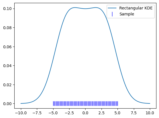
The boundaries of KDEs turn out to be a bit tricky: As a KDE approximates the sample density, the density outside of our sample goes to zero. This means that the KDE close to the boundaries will drop close to zero, as a KDE represents the accumulation of a “local average” density.
To demonstrate this, let’s use a perfect uniform kernel.
uniform_x = np.linspace(-5, 5, 70)
uniform_sample = zfit.Data.from_numpy(obs=obs_wide, array=uniform_x)
kde = zfit.pdf.KDE1DimExact(uniform_sample)

plt.plot(x, kde.pdf(x), label='Rectangular KDE')
plt.plot(uniform_x, np.zeros_like(uniform_x), 'b|', ms=12, label='Sample')
plt.legend()
<matplotlib.legend.Legend at 0x771ac42de390>
obs = zfit.Space('x', (-2, 0.5))  # will cut of data at -2, 0.5
data_narrow = gauss.sample(1000, limits=obs)

kde = zfit.pdf.KDE1DimExact(data_narrow)

x = np.linspace(-2, 0.5, 200)
plt.plot(x, kde.pdf(x), label='Biased KDE')
plt.plot(x, gauss.pdf(x, obs), label='True PDF')
plt.legend()
<matplotlib.legend.Legend at 0x771abe795ca0>
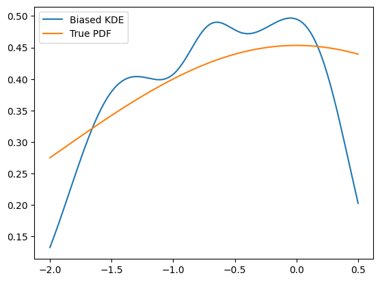
While this is maybe not a surprise, this means that if we’re only interested in the region of the sample, the KDE goes to zero too early. To illustrate, let’s zoom in into the region of our sample. Then the PDF looks like this:
plt.plot(uniform_x, kde.pdf(uniform_x), label='Rectangular KDE')
plt.plot(uniform_x, np.ones_like(uniform_x) / 10, label='True shape')
plt.plot(uniform_x, np.zeros_like(uniform_x), 'b|', ms=12, label='Sample')
plt.legend()
<matplotlib.legend.Legend at 0x771abe7bfa40>
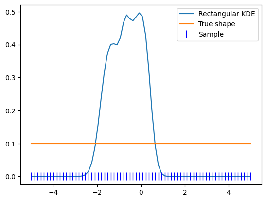
This effect is only a problem if the density of the sample itself does not go to zero by itself within our range of interest.
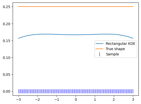
Wider data#
If the dataset that we have goes further than our PDF is meant to go, the best strategy is to simply provide a larger datasample.
The PDF takes an obs argument, which tells the “default space” and, most importantly, the normalization range. This does not need to coincide with the range of the given sample set, only the name of the obs has to.
Let’s define our PDF in a smaller range therefore.
limits_narrow = (-3, 3)
obs_narrow = zfit.Space('x', limits_narrow)

kde = zfit.pdf.KDE1DimExact(uniform_sample, obs=obs_narrow)

x_narrow = np.linspace(-3, 3, 100)
plt.plot(x_narrow, kde.pdf(x_narrow), label='Rectangular KDE')
plt.plot(x_narrow, np.ones_like(x_narrow) / 4, label='True shape')
plt.plot(x_narrow, np.zeros_like(x_narrow), 'b|', ms=12, label='Sample')
plt.legend()
<matplotlib.legend.Legend at 0x771abe627410>
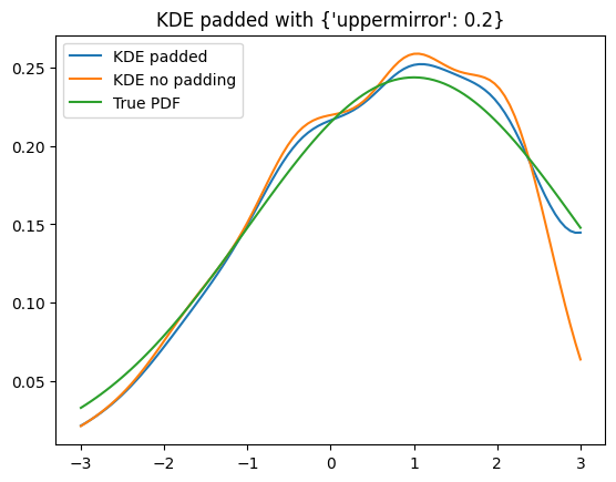
Padding#
As we don’t always have simply more data points outside of our region, the outside of the PDF can be padded in a different way: by mirroring the boundaries. This is effectively achieved by mirroring the dataset and can also be done manually.
The padding argument takes either a single float or a dict with “lowermirror” and/or “uppermirror” matched to a float to control mirroring the data on the lower respectively on the upper boundary of the data using. The number determines the fraction (in terms of difference between upper and lower boundary) of data that will be reflected.
This is effectively the same as requireing derivatives of zero at the boundary. While this helps lower the bias at the boundary, it is not a perfect solution.
gauss = zfit.pdf.Gauss(obs=obs_narrow, mu=1, sigma=2)
sample = gauss.sample(2000)
sample_np = zfit.run(sample.value())
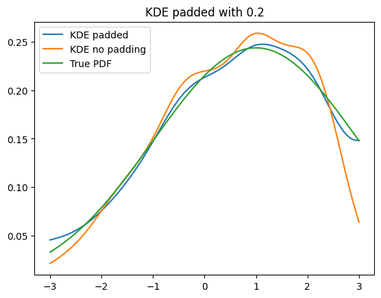
padding = 0.2
kde = zfit.pdf.KDE1DimExact(sample)
for pad in [{'uppermirror': 0.2}, padding]:
kde_padded = zfit.pdf.KDE1DimExact(sample, padding=pad)
plt.figure()
plt.title(f'KDE padded with {pad}')
plt.plot(x_narrow, kde_padded.pdf(x_narrow), label='KDE padded')
plt.plot(x_narrow, kde.pdf(x_narrow), label='KDE no padding')
plt.plot(x_narrow, gauss.pdf(x_narrow), label='True PDF')
plt.legend()
As the PDF is not truncated on the edges but the sample data is effectively modified, we can plot the PDF in a larger range, which makes the effects visible.
x_medium = np.linspace(-5, 5, 200)

plt.plot(x_medium, kde_padded.pdf(x_medium), label='KDE padded')
plt.plot(x_medium, kde.pdf(x_medium), label='KDE no padding')
plt.plot(x_medium, gauss.pdf(x_medium), label='True PDF')
width = (limits_narrow[1] - limits_narrow[0]) * padding
plt.bar([-3 - width, 3], height=[0.08, 0.2], width=width, align='edge', alpha=0.3, color='red', label="Mirrored data")
plt.legend()
<matplotlib.legend.Legend at 0x771abe794560>
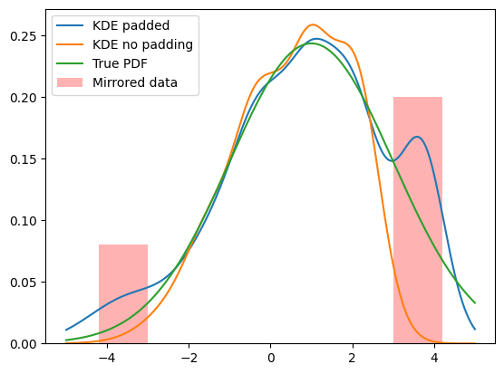
As can be seen, the mirrored data creates peaks which distorts our KDE. At the same time, it improves the shape in our region of interest.
Conclusion#
KDE suffers inherently from a boundary bias because the function inside our region of interest is affected by the kernels – or the lack thereof – outside of our region of interest.
If the PDF (=approximate sample size density) goes to zero inside our region of interest, we’re not affected.
Otherwise having a data sample that is larger than our region of interest is the best approach.
obsof a PDF can be different from thedataargument.If no data is available beyond the borders, an ad-hoc method is to mirror the data on the boundary, resulting in an (approximate) zero gradient condition, preventing the PDF from going towards zero too fast. This however changes the shape of the KDE outside of our region of interest. However, if the density does not go to zero at the boundary, the region beyond the boundary should usually anyway not be used.
Large sample KDE#
The exact KDE works well for smaller (~hundreds to thousands) of points, but becomes increasingly computationally demanding and is unfeasible for larger datasets. This computational demand can be reduced by a reduced number of sample points that can be achieved by binning the sample first.
Other approaches bin the data directly and then use it do estimate the density.
Grid KDE#
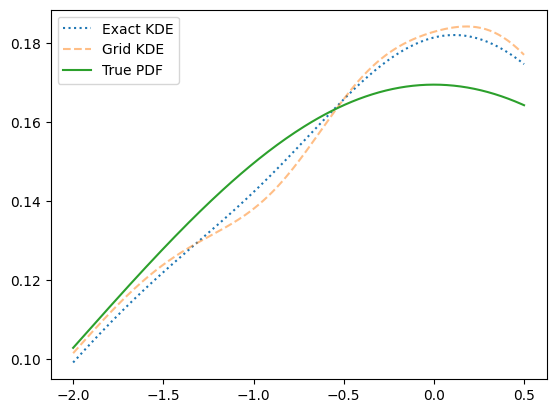
This implementation is almost the same as the exakt KDE expept that it bins the data first. So any argument that the KDE1DimExact takes and effect that applies to it are also valid for the KDE1DimExact.
Plotting the two, they lay pretty precisely on top of each and we don’t really loose by binning the PDF. This has two main reasons, the number of grid points and the binning method.
sample = true_pdf.sample(1000)
sample_np = zfit.run(sample.value())


kde_exact = zfit.pdf.KDE1DimExact(sample)
kde = zfit.pdf.KDE1DimGrid(sample)
plt.plot(x, kde_exact.pdf(x), ':', label='Exact KDE')
plt.plot(x, kde.pdf(x), '--', label='Grid KDE', alpha=0.5)
plt.plot(x, true_pdf.pdf(x), label='True PDF')
plt.legend()
<matplotlib.legend.Legend at 0x771abe539070>
Number of grid points#
By default, the num_grid_points is set to a comparably large numbe around 256-1024. This creates a very fine binning of the space and renders the information loss due to binning nearly neglectable.
This number can be adjusted, mainly to reduce the computational cost which is directly proportional to the number of grid points.
for num_grid_points in [5, 10, 20, 100, 1024]:
    kde = zfit.pdf.KDE1DimGrid(sample, num_grid_points=num_grid_points)

    plt.plot(x_medium, kde.pdf(x_medium), '--', label=f'n={num_grid_points}')
#     plt.plot(x, true_pdf.pdf(x), label='True PDF')
plt.plot(x_medium, kde_exact.pdf(x_medium), label='Exact KDE', alpha=0.3, linewidth=7)
plt.legend()
<matplotlib.legend.Legend at 0x771a9f611070>
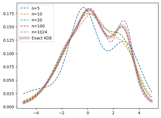
For a small number of bins, the approximation breaks down, but for a larger number, it is as good as the exact KDE.
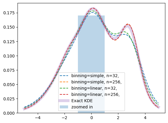
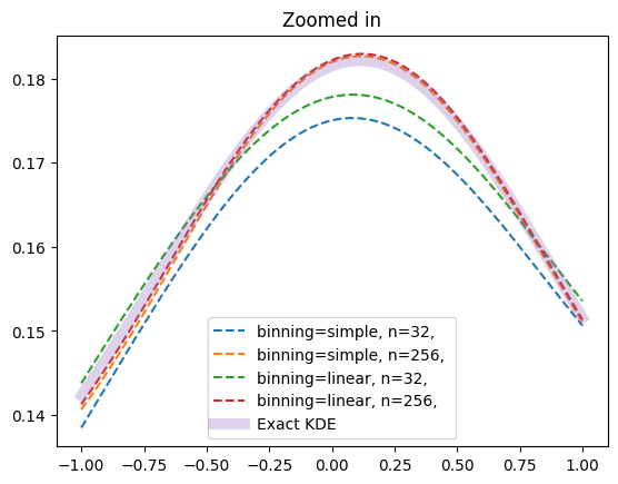
Binning method#
Binning is the process of filling data points into bins or buckets. Simple binning that is used in classical histograms means that each bin receives plus one count for each event (or plus the event weight in case of weights) falling within the bin edges while the neighbouring bins do not get any count. This can lead to fluctuating bins, as an event close to the bin edges actually lies “in the middle of two bins”.
To reduce this fluctuation, zfit implements additionally linear binning. This method assigns a fraction of the whole weight to both grid points (bins) on either side, proportional to the closeness of grid point and data point, e.g. the distance between grid points (bin width).
plt.bar([-1], height=0.17, width=2, align='edge', alpha=0.3, label='zoomed in')
x_tiny = np.linspace(-1, 1, 200)
for title, xplot in [('',x_medium), ('Zoomed in', x_tiny)]:
    plt.title(title)
    for binning_method in ['simple', 'linear']:
        for num_grid_points in [32, 256]:

            kde = zfit.pdf.KDE1DimGrid(sample, num_grid_points=num_grid_points, binning_method=binning_method)

            plt.plot(xplot, kde.pdf(xplot), '--', label=f'binning={binning_method}, n={num_grid_points}, ')
    #     plt.plot(x, true_pdf.pdf(x), label='True PDF')
    plt.plot(xplot, kde_exact.pdf(xplot), label='Exact KDE', alpha=0.3, linewidth=7)
    plt.legend()
    plt.figure()
<Figure size 640x480 with 0 Axes>
Linear binning is smoother than the simple binning and follows closer the exact PDF, although the effect is rather small in our example with the standard number of grid points. For less grid points, the effect becomes significant and the improvement of linear binning allows an accurate KDE with a minimal number of grid points.
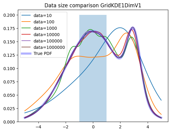
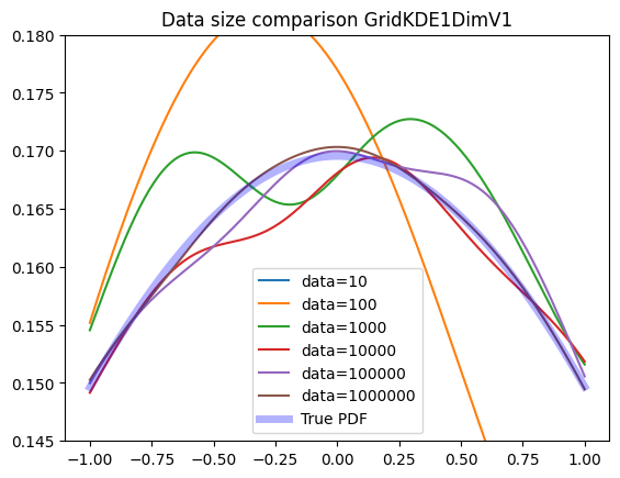
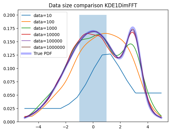
Data size#
The Grid KDE is able to handle large amounts of data with a similar evaluation time.
def plot_large(kdetype, npower=6):
    sample_sizes = 10 ** np.linspace(1, npower, npower)
    for n in sample_sizes:
        n = int(n)
        for i, xplot in enumerate([x_medium, x_tiny]):
            plt.figure(i)
            sample = true_pdf.sample(n)
            kde = kdetype(sample)

            plt.plot(xplot, kde.pdf(xplot), label=f'data={n}')
            if n == sample_sizes[-1]:
                plt.title(f'Data size comparison {kde.name}')
                plt.plot(xplot, true_pdf.pdf(xplot), 'b', label='True PDF', alpha=0.3, linewidth=5)
                plt.legend()
                if i == 0:
                    plt.bar([-1], height=0.2, width=2, align='edge', alpha=0.3, label='zoomed in')
                else:
                    plt.gca().set_ylim((0.145, 0.18))
plot_large(zfit.pdf.KDE1DimGrid)
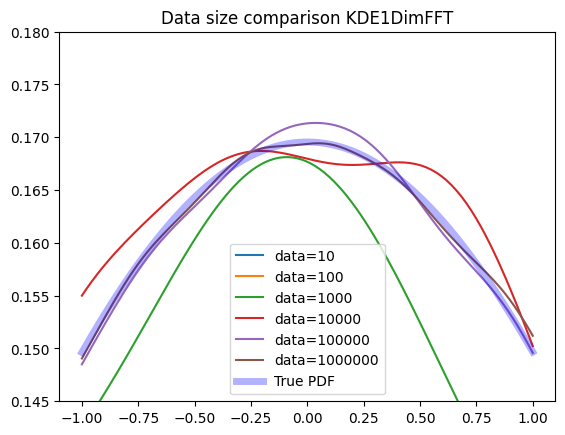
FFT KDE#
Another technique to speed up the computation is to rewrite the kernel density estimation as convolution operation between the kernel function and the grid counts (bin counts). Since this method relies on the discrete Fourier transform, the result is an interpolation.
By using the fact that a convolution is just a multiplication in Fourier space and only evaluating the KDE at grid points one can reduce the computational complexity down to \(\mathcal{O}(\log{N} \cdot N)\).
plot_large(zfit.pdf.KDE1DimFFT)
Improved Sheather-Jones Algorithm#
A different take on KDEs is the improved Sheather-Jones (ISJ) algorithm. It is an adaptive kernel density estimator based on linear diffusion processes, where the optimality is treated as solving the heat equation. This algorith also includes an estimation for the optimal bandwidth of a normal KDE (and can be used in the exact and grid KDE as "isj").
This yields discrete points, so the result is an interpolation.
plot_large(zfit.pdf.KDE1DimISJ)
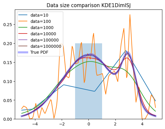
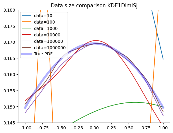
The ISJ algorithm is rather wiggly for smaller datasets and tends to overfit while delivering great performance with larger datasets.
KDE comparison for large data#
sample_size = 300_000
kde_grid = zfit.pdf.KDE1DimGrid
kde_fft = zfit.pdf.KDE1DimFFT
kde_isj = zfit.pdf.KDE1DimISJ
for i, xplot in enumerate([x_medium,x_tiny/5 + 3]):
    plt.figure(i)
    sample = true_pdf.sample(sample_size)
    for kdetype, linestyle in [
        (kde_grid, '-.'),
                    (kde_fft, ':'),
                    (kde_isj, '--')
                   ]:
        kde = kdetype(sample, num_grid_points=1024)
        plt.plot(xplot, kde.pdf(xplot),linestyle, label=f'{kde.name}')

    plt.title(f'Large data KDE comparison')
    plt.plot(xplot, true_pdf.pdf(xplot), 'b', label='True PDF', alpha=0.3, linewidth=5)
    plt.legend()
    if i == 0:
        width = 2 / 5
        plt.bar([3], height=0.185, width=width, alpha=0.3, label='zoomed in')
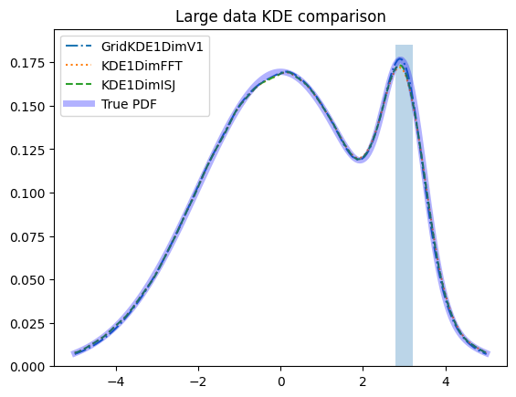
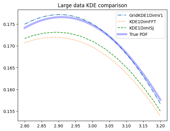
As we can see, the PDFs all perform nearly equally well for large datasets.