Combining measurements

When we do a fit, we can have additional knowledge about a parameter from other measurements. This can be taken into account either through a simultaneous fit or by adding a constraint (subsidiary measurement).

Adding a constraint

If we know a parameters value from a different measurement and want to constraint this using its uncertainty, a Gaussian constraint can be added to the likelihood as

(1)\[\begin{align} \mathrm{constr_i} = \mathrm{Gauss}(\mu_{measured}; \theta_i, \sigma_{measured}) \end{align}\]

In general, additional terms can be added to the likelihood arbitrarily in zfit, be it to incorporate other shaped measurements or to add penalty terms to confine a fit within boundaries.

import hepunits as u
import matplotlib.pyplot as plt
import mplhep
import numpy as np
import particle.literals as lp
import tensorflow as tf
import zfit.z.numpy

plt.rcParams['figure.figsize'] = (8, 6)

mu_true = lp.B_plus.mass * u.MeV
sigma_true = 50 * u.MeV

# number of signal and background
n_sig_rare = 120
n_bkg_rare = 700

# create some data
signal_np = np.random.normal(loc=mu_true, scale=sigma_true, size=n_sig_rare)
bkg_np_raw = np.random.exponential(size=20000, scale=700)
bkg_np = bkg_np_raw[bkg_np_raw < 1000][:n_bkg_rare] + 5000  # just cutting right, but zfit could also cut

# Firstly, the observable and its range is defined
obs = zfit.Space('Bmass', 5000, 6000)  # for whole range

# load data into zfit and let zfit concatenate the data
signal_data = zfit.Data(signal_np, obs=obs)
bkg_data = zfit.Data(bkg_np, obs=obs)
data = zfit.data.concat([signal_data, bkg_data])
# (we could also do it manually)
# data = zfit.Data(array=np.concatenate([signal_np, bkg_np], axis=0), obs=obs)

# Parameters are specified:  (name (unique), initial, lower, upper) whereas lower, upper are optional
mu = zfit.Parameter('mu', 5279, 5100, 5400)
sigma = zfit.Parameter('sigma', 20, 1, 200)
sig_yield = zfit.Parameter('sig_yield', n_sig_rare + 30,
                           step_size=3)  # step size: default is small, use appropriate
signal = zfit.pdf.Gauss(mu=mu, sigma=sigma, obs=obs, extended=sig_yield)

lam = zfit.Parameter('lambda', -0.002, -0.1, -0.00001, step_size=0.001)  # floating, also without limits
bkg_yield = zfit.Parameter('bkg_yield', n_bkg_rare - 40, step_size=1)
comb_bkg = zfit.pdf.Exponential(lam, obs=obs, extended=bkg_yield)

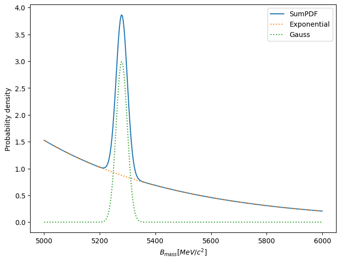
# The final model is the combination of the signal and backgrond PDF
model = zfit.pdf.SumPDF([comb_bkg, signal])

constraint = zfit.constraint.GaussianConstraint(mu, observation=5275 * u.MeV, sigma=15 * u.MeV)

nll = zfit.loss.ExtendedUnbinnedNLL(model, data, constraints=constraint)
minimizer = zfit.minimize.Minuit(gradient="zfit")
result = minimizer.minimize(nll)
result.hesse();

print(result)

FitResult

 of
<ExtendedUnbinnedNLL model=[<zfit.<class 'zfit.models.functor.SumPDF'>  params=[Composed_autoparam_1, Composed_autoparam_2]] data=[<zfit.Data: Data obs=('Bmass',) shape=(820, 1)>] constraints=[<zfit.core.constraint.GaussianConstraint object at 0x7fca16e6b190>]> 
with
<Minuit Minuit tol=0.001>

╒═════════╤═════════════╤══════════════════╤═════════╤══════════════════════════════╕
│  valid  │  converged  │  param at limit  │   edm   │   approx. fmin (full | opt.) │
╞═════════╪═════════════╪══════════════════╪═════════╪══════════════════════════════╡
│  

True

   │    True

     │      False

       │ 0.00018 │           866.35 |  9979.792 │
╘═════════╧═════════════╧══════════════════╧═════════╧══════════════════════════════╛

Parameters

name         value  (rounded)        hesse    at limit
---------  ------------------  -----------  ----------
bkg_yield             729.034  +/-      32       False

sig_yield              91.117  +/-      20       False

lambda             -0.0016528  +/- 0.00014       False

mu                    5284.01  +/-     7.6       False

sigma                 39.4786  +/-     9.2       False

Simultaneous fits

Sometimes, we don’t want to fit a single channel but multiple with the same likelihood and having shared parameters between them. In this example, we will fit the decay simultaneously to its resonant control channel.

A simultaneous likelihood is the product of different likelihoods defined by

(2)\[\begin{align} \mathcal{L}_{f(x)}(\theta | {data_0, data_1, ..., data_n}) &= \prod_{i=1}^{n} \mathcal{L}(\theta_i, data_i) \end{align}\]

and becomes in the NLL a sum

(3)\[\begin{align} \mathrm{NLL}_{f(x)}(\theta | {data_0, data_1, ..., data_n}) &= \sum_{i=1}^{n} \mathrm{NLL}(\theta_i, data_i) \end{align}\]

n_sig_reso = 40000
n_bkg_reso = 3000

# create some data
signal_np_reso = np.random.normal(loc=mu_true, scale=sigma_true * 0.7, size=n_sig_reso)
bkg_np_raw_reso = np.random.exponential(size=20000, scale=900)
bkg_np_reso = bkg_np_raw_reso[bkg_np_raw_reso < 1000][:n_bkg_reso] + 5000

# load data into zfit
obs_reso = zfit.Space('Bmass_reso', 5000, 6000)
signal_data_reso = zfit.Data(signal_np_reso, obs=obs_reso)
bkg_data_reso = zfit.Data(bkg_np_reso, obs=obs_reso)
data_reso = zfit.data.concat([signal_data_reso, bkg_data_reso])

Sharing and composing parameters

As an example, the same signal shape will be used with the identical mu yet a scaled sigma. This means that the sigma of our control mode corresponds to the sigma of our signal times a scaling parameter. Therefore, the scaled_sigma is a function of two other parameters, sigma and sigma_scaling and cannot change it’s value independently. There are two fundamentally distinct types to represent this behavior in zfit, independent (Parameter) and dependent parameters (ComplexParameter, ComposedParameter,…)

Independent parameter

An independent parameter has, as a distinctive method, a set_value that changes the value of the parameter. In a fit, or in general, these are the only object that can directly change their value and therefore do not depend on other objects while most other objects depend on Parameters. As a consequence, this parameters can have limits (which effectively restrict the possible values a Parameter can be assigned to) and have a step_size, a hint to any minimization algorithm about the order of magnitude that a change in the parameter will have on the loss.

Another attribute is a floating flag: if set to False, the parameter won’t be floating in the fit, whether explicitly given or implicitly inferred from the dependencies.

Dependent parameter

These are single-valued functions effectively that depend on other objects, usually other parameters. Therefore, a dependent parameter does not have a set_value function and also does not posses limits. The latter is preferred to be set with the Parameter it depends on, however, if a hard limit is required, this can always be enforced in the definition of a ComposedParameter.

The most notable parameter is the ComposedParameter, which returns an arbitrary function of its input arguments, the latter which can be specified with the params argument.

While this parameters cannot change there value explicitly and therefore won’t be used by a minimizer, the zfit minimizers automatically extract the independent parameters that a dependent parameter depends on (if this is given as an argument.)

As a consequence, these parameters also miss a step_size attribute. Furthermore, floating can’t be used, neither set nor retrieved; it is rather advised to check directly with its dependencies.

Sharing parameters

Since in zfit, every parameter object is unique, also defined by its name, it is straightforward to know when a parameter is shared in the loss and when it is not: if the same object is used in two places, it is shared. This can be arbitrarily mixed.

# Firstly, we create a free scaling parameter
sigma_scaling = zfit.Parameter('sigma_scaling', 0.9, 0.1, 10, step_size=0.1)


def sigma_scaled_fn(sigma, sigma_scaling):
    return sigma * sigma_scaling  # this can be an arbitrary function


sigma_scaled = zfit.ComposedParameter('sigma scaled',  # name
                                      sigma_scaled_fn,  # function
                                      params=[sigma, sigma_scaling],  # the objects used inside the function
                                      unpack_params=True  # we could also just use a `params` argument, a dict
                                      )

reso_sig_yield = zfit.Parameter('reso_sig_yield', n_sig_reso - 100, 0, n_sig_reso * 3,
                                step_size=1)
signal_reso = zfit.pdf.Gauss(mu=mu,  # the same as for the rare mode
                             sigma=sigma_scaled,
                             obs=obs_reso,
                             extended=reso_sig_yield)

lambda_reso = zfit.Parameter('lambda_reso', -0.002, -0.01, 0.0001)
reso_bkg_yield = zfit.Parameter('reso_bkg_yield', n_bkg_reso + 70, 0, 2e5, step_size=1)
comb_bkg_reso = zfit.pdf.Exponential(lambda_reso, obs=obs_reso, extended=reso_bkg_yield)


model_reso = zfit.pdf.SumPDF([comb_bkg_reso, signal_reso])

To implement the simultaneous fit, there are two ways to achieve this in zfit. As an important distinction to other frameworks, zfit translates the above equation

(4)\[\begin{align} \mathrm{NLL}_{f(x)}(\theta | {data_0, data_1, ..., data_n}) &= \sum_{i=1}^{n} \mathrm{NLL}(\theta_i, data_i) \end{align}\]

directly into code.

We can build two losses and add them directly or give a list of models and data, which build a loss each one and add up.

nll_rare = zfit.loss.ExtendedUnbinnedNLL(model, data)
nll_reso = zfit.loss.ExtendedUnbinnedNLL(model_reso, data_reso)
nll_simultaneous = nll_rare + nll_reso

signal_reso.get_yield()

<zfit.Parameter 'reso_sig_yield' floating=True value=3.99e+04>

result_simultaneous = minimizer.minimize(nll_simultaneous)

result_simultaneous.hesse()

{<zfit.Parameter 'bkg_yield' floating=True value=728.1>: {'error': 30.614611194141823,
  'cl': 0.68268949},
 <zfit.Parameter 'sig_yield' floating=True value=91.95>: {'error': 17.39989772395696,
  'cl': 0.68268949},
 <zfit.Parameter 'lambda' floating=True value=-0.001645>: {'error': 0.00013926549894174853,
  'cl': 0.68268949},
 <zfit.Parameter 'mu' floating=True value=5279>: {'error': 0.18092146027043224,
  'cl': 0.68268949},
 <zfit.Parameter 'sigma' floating=True value=40.53>: {'error': 4.193087191942704,
  'cl': 0.68268949},
 <zfit.Parameter 'reso_bkg_yield' floating=True value=2961>: {'error': 65.0304002889996,
  'cl': 0.68268949},
 <zfit.Parameter 'reso_sig_yield' floating=True value=4.004e+04>: {'error': 203.24943946602693,
  'cl': 0.68268949},
 <zfit.Parameter 'lambda_reso' floating=True value=-0.0009567>: {'error': 6.919553630461632e-05,
  'cl': 0.68268949},
 <zfit.Parameter 'sigma_scaling' floating=True value=0.863>: {'error': 0.08929991434150471,
  'cl': 0.68268949}}

print(result_simultaneous.params)

name              value  (rounded)        hesse    at limit
--------------  ------------------  -----------  ----------
bkg_yield                  728.101  +/-      31       False

sig_yield                  91.9548  +/-      17       False

lambda                 -0.00164534  +/- 0.00014       False

mu                         5279.42  +/-    0.18       False

sigma                      40.5266  +/-     4.2       False

reso_bkg_yield             2961.19  +/-      65       False

reso_sig_yield             40040.9  +/-   2e+02       False

lambda_reso            -0.00095675  +/- 6.9e-05       False

sigma_scaling             0.862959  +/-   0.089       False

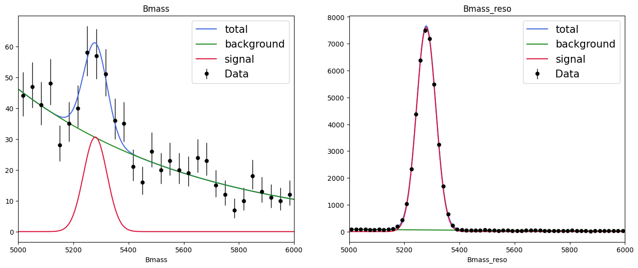
Plotting a simultaneous loss

Since the definition of a simultaneous fit is as above, it is simple to plot each component separately: either my using the attributes of the loss to access the models and plot in a general fashion or directly reuse the model and data from before; we created them manually before.

# Sets the values of the parameters to the result of the simultaneous fit
# in case they were modified.
zfit.param.set_values(nll_simultaneous.get_params(), result_simultaneous)


def plot_fit_projection(model, data, nbins=30, ax=None):
    # The function will be reused.
    if ax is None:
        ax = plt.gca()

    lower, upper = data.data_range.limit1d

    # Creates and histogram of the data and plots it with mplhep.
    counts, bin_edges = np.histogram(data.unstack_x(), bins=nbins)
    mplhep.histplot(counts, bins=bin_edges, histtype="errorbar", yerr=True,
                    label="Data", ax=ax, color="black")

    binwidth = np.diff(bin_edges)[0]
    x = tf.linspace(lower, upper, num=1000)  # or np.linspace

    # Line plots of the total pdf and the sub-pdfs.
    y = model.ext_pdf(x) * binwidth
    ax.plot(x, y, label="total", color="royalblue")
    for m, l, c in zip(model.get_models(), ["background", "signal"], ["forestgreen", "crimson"]):
        ym = m.ext_pdf(x) * binwidth
        ax.plot(x, ym, label=l, color=c)

    ax.set_title(data.data_range.obs[0])
    ax.set_xlim(lower, upper)
    ax.legend(fontsize=15)

    return ax


fig, axs = plt.subplots(1, 2, figsize=(16, 6))

for mod, dat, ax, nb in zip(nll_simultaneous.model, nll_simultaneous.data, axs, [30, 60]):
    plot_fit_projection(mod, dat, nbins=nb, ax=ax)

Discovery test

We observed an excess of our signal:

print(result_simultaneous.params[sig_yield])

{'value': 91.95480704554072, 'hesse': {'error': 17.39989772395696, 'cl': 0.68268949}}

Now we would like to compute the significance of this observation or, in other words, the probabilty that this observation is the result of the statistical fluctuation. To do so we have to perform an hypothesis test where the null and alternative hypotheses are defined as:

• \(H_{0}\), the null or background only hypothesis, i.e. \(N_{sig} = 0\);

• \(H_{1}\), the alternative hypothesis, i.e \(N_{sig} = \hat{N}_{sig}\), where \(\hat{N}_{sig}\) is the fitted value of \(N_{sig}\) printed above.

In hepstats to formulate a hypothesis you have to use the POI (Parameter Of Interest) class.

from hepstats.hypotests.parameters import POI

# the null hypothesis
sig_yield_poi = POI(sig_yield, 0)

What the POI class does is to take as input a zfit.Parameter instance and a value corresponding to a given hypothesis. You can notice that we didn’t define here the alternative hypothesis as in the discovery test the value of POI for alternate is set to the best fit value.

The test statistic used is the profile likelihood ratio and defined as:

(5)\[\begin{equation} q_{0} = \left\{ \begin{array}{ll} -2 \ln \frac{\mathcal{L}(N_{sig}=0, \; \hat{\hat{\theta}})}{\mathcal{L}(N_{sig}=\hat{N}_{sig}, \; \hat{\theta})} & \mbox{if } \; \hat{N}_{sig} \geq 0 \\ 0 & \mbox{if } \; \hat{N}_{sig} < 0 \end{array} \right. \end{equation}\]

where \(\hat{\theta}\) are the best fitted values of the nuisances parameters (i.e. background yield, exponential slope…), while \(\hat{\hat{\theta}}\) are the fitted values of the nuisances when \({N}_{sig} = 0\).

From the test statistic distribution a p-value can computed as

(6)\[\begin{equation} p_{0} = \int_{q_{0}^{obs}}^{\infty} f(q_{0} |H_{0}) dq_{0} \end{equation}\]

where \(q_{0}^{obs}\) is the value of the test statistic evaluated on observed data.

The construction of the test statistic and the computation of the p-value is done in a Calculator object in hepstats. In this example we will use in this example the AsymptoticCalculator calculator which assumes that \(q_{0}\) follows a \(\chi^2(ndof=1)\) which simplifies the p-value computation to

(7)\[\begin{equation} p_{0} = 1 - \Phi\bigg({\sqrt{q_{0}^{obs}}}\bigg). \end{equation}\]

The calculator objects takes as input the likelihood function and a minimizer to profile the likelihood.

from hepstats.hypotests.calculators import AsymptoticCalculator

# construction of the calculator instance
calculator = AsymptoticCalculator(input=nll_simultaneous, minimizer=minimizer)
calculator.bestfit = result_simultaneous

# equivalent to above
calculator = AsymptoticCalculator(input=result_simultaneous, minimizer=minimizer)

There is another calculator in hepstats called FrequentistCalculator which constructs the test statistic distribution \(f(q_{0} |H_{0})\) with pseudo-experiments (toys), but it takes more time.

The Discovery class is a high-level class that takes as input a calculator and a POI instance representing the null hypothesis, it basically asks the calculator to compute the p-value and also computes the signifance as

(8)\[\begin{equation} Z = \Phi^{-1}(1 - p_0). \end{equation}\]

from hepstats.hypotests import Discovery

discovery = Discovery(calculator=calculator, poinull=sig_yield_poi)
discovery.result()

p_value for the Null hypothesis = 2.2687673961740984e-10

Significance (in units of sigma) = 6.2343169775013285

(2.2687673961740984e-10, 6.2343169775013285)

So we get a significance of about \(7\sigma\) which is well above the \(5 \sigma\) threshold for discoveries 😃.

Upper limit calculation

Let’s try to compute the discovery significance with a lower number of generated signal events.

# Sets the values of the parameters to the result of the simultaneous fit
zfit.param.set_values(nll_simultaneous.get_params(), result_simultaneous)
sigma_scaling.floating = False

# Creates a sampler that will draw events from the model
sampler = model.create_sampler()

# Creates new simultaneous loss
nll_simultaneous_low_sig = zfit.loss.ExtendedUnbinnedNLL(model, sampler) + nll_reso

# Samples with sig_yield = 10. Since the model is extended the number of
# signal generated is drawn from a poisson distribution with lambda = 10.
sampler.resample({sig_yield: 10})

calculator_low_sig = AsymptoticCalculator(input=nll_simultaneous_low_sig, minimizer=minimizer)

discovery_low_sig = Discovery(calculator=calculator_low_sig, poinull=sig_yield_poi)
discovery_low_sig.result()
print(f"\n {calculator_low_sig.bestfit.params} \n")

Get fit best values!

W MnHesse Analytical calculator  	[  -1.69814812e-05 -2.025312624e-05    -0.0509158992    -0.1702872609    0.03751929868    -0.2524187955    0.01524917472    0.01348904981]	  numerical  	[ -1.726421058e-05   -3.2894097e-05   -0.05831339971    -0.1745895082    0.03253207527    -0.2524915913    0.01524631393    0.01039098984]	  g2  	[   0.001333849566    0.00689583839      8902.009533      661422.6047      253630.8392      146990.7316       78459.2199      2072.924895]	

p_value for the Null hypothesis = 0.30336501365699386

Significance (in units of sigma) = 0.5147467113695439

 name              value  (rounded)    at limit
--------------  ------------------  ----------
bkg_yield                  743.152       False

sig_yield                  6.83483       False

lambda                 -0.00168844       False

mu                         5279.42       False

sigma                      40.5315       False

reso_bkg_yield             2960.89       False

reso_sig_yield             40039.1       False

lambda_reso           -0.000955933       False

We might consider computing an upper limit on the signal yield instead. The test statistic for an upper limit calculation is

(9)\[\begin{equation} q_{N_{sig}} = \left\{ \begin{array}{ll} -2 \ln \frac{\mathcal{L}(N_{sig}, \; \hat{\hat{\theta}})}{\mathcal{L}(N_{sig}=\hat{N}_{sig}, \; \hat{\theta})} & \mbox{if } \; \hat{N}_{sig} \leq N_{sig} \\ 0 & \mbox{if } \; \hat{N}_{sig} > N_{sig}. \end{array} \right. \end{equation}\]

and the p-value is

(10)\[\begin{equation} p_{N_{sig}} = \int_{q_{N_{sig}}^{obs}}^{\infty} f(q_{N_{sig}} |N_{sig}) dq_{N_{sig}}. \end{equation}\]

The upper limit on \(N_{sig}\), \(N_{sig, \uparrow}\) is found for \(p_{N_{sig, \uparrow}} = 1 - \alpha\), \(\alpha\) being the confidence level (typically \(95 \%\)). The upper limit is found by interpolation of the p-values as a function of \(N_{sig}\), which is done the UpperLimit class. We have to give the range of values of \(N_{sig}\) to scan using the POIarray class which as the POI class takes as input the parameter but takes several values to evaluate the parameter instead of one.

from hepstats.hypotests import UpperLimit
from hepstats.hypotests.parameters import POIarray

#Background only hypothesis.
bkg_only = POI(sig_yield, 0)
# Range of Nsig values to scan.
sig_yield_scan = POIarray(sig_yield, np.linspace(0, 70, 10))

ul = UpperLimit(calculator=calculator_low_sig, poinull=sig_yield_scan, poialt=bkg_only)
ul.upperlimit(alpha=0.05);

Get fitted values of the nuisance parameters for the alternative hypothesis!

FitResult

 of
<ExtendedBinnedNLL model=[<zfit.models.tobinned.BinnedFromUnbinnedPDF object at 0x7fc9fba32290>, <zfit.models.tobinned.BinnedFromUnbinnedPDF object at 0x7fc9fbb5aa10>] data=[<zfit._data.binneddatav1.BinnedData object at 0x7fca02302210>, <zfit._data.binneddatav1.BinnedData object at 0x7fc9fbf31b50>] constraints=[]> 
with
<Minuit Minuit tol=0.001>

╒═════════╤═════════════╤══════════════════╤═════════╤══════════════════════════════╕
│  valid  │  converged  │  param at limit  │   edm   │   approx. fmin (full | opt.) │
╞═════════╪═════════════╪══════════════════╪═════════╪══════════════════════════════╡
│  

True

   │    True

     │      False

       │ 7.2e-05 │       -288679.11 | -287313.7 │
╘═════════╧═════════════╧══════════════════╧═════════╧══════════════════════════════╛

Parameters

name              value  (rounded)    at limit
--------------  ------------------  ----------
bkg_yield                  749.943       False

lambda                 -0.00169807       False

mu                         5279.42       False

sigma                      40.5415       False

reso_bkg_yield             2962.38       False

reso_sig_yield               40038       False

lambda_reso             -0.0009551       False

Observed upper limit: sig_yield = 32.43994223209022

Expected upper limit: sig_yield = 27.26225533489645

Expected upper limit +1 sigma: sig_yield = 38.66791298913074

Expected upper limit -1 sigma: sig_yield = 19.34122302338897

Expected upper limit +2 sigma: sig_yield = 53.0391889049599

Expected upper limit -2 sigma: sig_yield = 14.07008627303169

from utils import plotlimit

plotlimit(ul, CLs=False)

<Axes: xlabel='parameter of interest', ylabel='p-value'>

Splot

This is now an demonstration of the sPlot algorithm, described in Pivk:2004ty.

If a data sample is populated by different sources of events, like signal and background, sPlot is able to unfold the contributions of the different sources for a given variable.

Let’s construct a dataset with two variables, the invariant mass and lifetime, for the resonant signal defined above and the combinatorial background.

# Signal distributions.
nsig_sw = 20000
np_sig_m_sw = signal_reso.sample(nsig_sw)["Bmass_reso"]
np_sig_t_sw = np.random.exponential(size=nsig_sw, scale=1)

# Background distributions.
nbkg_sw = 150000
np_bkg_m_sw = comb_bkg_reso.sample(nbkg_sw)["Bmass_reso"]
np_bkg_t_sw = np.random.normal(size=nbkg_sw, loc=2.0, scale=2.5)

# Lifetime cut.
t_cut = np_bkg_t_sw > 0
np_bkg_t_sw = np_bkg_t_sw[t_cut]
np_bkg_m_sw = np_bkg_m_sw[t_cut]

# Mass distribution
np_m_sw = np.concatenate([np_sig_m_sw, np_bkg_m_sw])

# Lifetime distribution
np_t_sw = np.concatenate([np_sig_t_sw, np_bkg_t_sw])

# Plots the mass and lifetime distribution.
fig, axs = plt.subplots(1, 2, figsize=(16, 6))
axs[0].hist([np_bkg_m_sw, np_sig_m_sw], bins=50, stacked=True, label=("background", "signal"), alpha=.7)
axs[0].set_xlabel("m")
axs[0].legend(fontsize=15)
axs[1].hist([np_bkg_t_sw, np_sig_t_sw], bins=50, stacked=True, label=("background", "signal"), alpha=.7)
axs[1].set_xlabel("t")
axs[1].legend(fontsize=15);

In this particular example we want to unfold the signal lifetime distribution. To do so sPlot needs a discriminant variable to determine the yields of the various sources using an extended maximum likelihood fit.

# Builds the loss.
data_sw = zfit.Data(np_m_sw, obs=obs_reso)
nll_sw = zfit.loss.ExtendedUnbinnedNLL(model_reso, data_sw)

#This parameter was useful in the simultaneous fit but not anymore so we fix it.
sigma_scaling.floating = False

# Minimizes the loss.
result_sw = minimizer.minimize(nll_sw)
print(result_sw.params)

name              value  (rounded)    at limit
--------------  ------------------  ----------
reso_bkg_yield              117876       False

reso_sig_yield               20130       False

lambda_reso           -0.000957066       False

mu                         5278.99       False

sigma                      40.8382       False

# Visualization of the result.
zfit.param.set_values(nll_sw.get_params(), result_sw)
plot_fit_projection(model_reso, data_sw, nbins=100)

<Axes: title={'center': 'Bmass_reso'}>

sPlot will use the fitted yield for each sources to derive the so-called sWeights for each data point:

(11)\[\begin{equation} W_{n}(x) = \frac{\sum_{j=1}^{N_S} V_{nj} f_j(x)}{\sum_{k=1}^{N_S} N_{k}f_k(x)} \end{equation}\]

with

(12)\[\begin{equation} V_{nj}^{-1} = \sum_{e=1}^{N} \frac{f_n(x_e) f_j(x_e)}{(\sum_{k=1}^{N_S} N_{k}f_k(x))^2} \end{equation}\]

where \({N_S}\) is the number of sources in the data sample, here 2. The index \(n\) represents the source, for instance \(0\) is the signal and \(1\) is the background, then \(f_0\) and \(N_0\) are the pdf and yield for the signal.

In hepstats the sWeights are computed with the compute_sweights function which takes as arguments the fitted extended model and the discrimant data (on which the fit was performed).

from hepstats.splot import compute_sweights

weights = compute_sweights(model_reso, data_sw)

print(weights)

{<zfit.Parameter 'reso_bkg_yield' floating=True value=1.179e+05>: array([-0.15627   ,  0.30820479, -0.26438225, ...,  1.01417594,
        1.19939028,  0.42460686]), <zfit.Parameter 'reso_sig_yield' floating=True value=2.013e+04>: array([ 1.15625313,  0.69178573,  1.26436367, ..., -0.01417418,
       -0.19938558,  0.57538552])}

print("Sum of signal sWeights: ", np.sum(weights[reso_sig_yield]))
print("Sum of background sWeights: ", np.sum(weights[reso_bkg_yield]))

Sum of signal sWeights: 

20130.005173097292

Sum of background sWeights: 

117875.88586562786

Now we can apply the signal sWeights on the lifetime distribution and retrieve its signal components.

fig, axs = plt.subplots(1, 2, figsize=(16, 6))
nbins = 40

sorter = np_m_sw.argsort()

axs[0].plot(np_m_sw[sorter], weights[reso_sig_yield][sorter], label="$w_\\mathrm{sig}$")
axs[0].plot(np_m_sw[sorter], weights[reso_bkg_yield][sorter], label="$w_\\mathrm{bkg}$")
axs[0].plot(np_m_sw[sorter], weights[reso_sig_yield][sorter] + weights[reso_bkg_yield][sorter],
            "-k", label="$w_\\mathrm{sig} + w_\\mathrm{bkg}$")
axs[0].axhline(0, color="0.5")
axs[0].legend(fontsize=15)
axs[0].set_xlim(5000, 5600)

axs[1].hist(np_t_sw, bins=nbins, range=(0, 6), weights=weights[reso_sig_yield], label="weighted histogram", alpha=.5)
axs[1].hist(np_sig_t_sw, bins=nbins, range=(0, 6), histtype="step", label="true histogram", lw=1.5)
axs[1].set_xlabel("t")
axs[1].legend(fontsize=15);

Be careful the sPlot technique works only on variables that are uncorrelated with the discriminant variable.

print(f"Correlation between m and t: {np.corrcoef(np_m_sw, np_t_sw)[0, 1]}")

Correlation between m and t: 0.06903206265730294

Let’s apply to signal sWeights on the mass distribution to see how bad the results of sPlot is when applied on a variable that is correlated with the discrimant variable.

plt.hist(np_m_sw, bins=100, range=(5000, 6000), weights=weights[reso_sig_yield]);