Introduction to zfit

Introduction to zfit#

zfit is a model building and fitting library, mostly for likelihood fits and with advanced features for HEP analyses.

It aims to define an API and workflow to be the stable core and allow other libraries to be built on top of it. Furthermore, it uses JIT compilation and autograd (current backend TensorFlow, future JAX (?)) to significantly speed up the computation.

Workflow#

There are five mostly independent parts in zfit zfit workflow

import matplotlib.pyplot as plt
import mplhep
import numpy as np
import zfit
# znp is a subset of numpy functions with a numpy interface but using actually the zfit backend (currently TF)
import zfit.z.numpy as znp
import zfit_physics as zphysics  # extension (for user contribution) containing physics PDFs
from zfit import z  # z is the backend, for gradients, JIT etc

No module named 'nlopt'

Data#

This component in general plays a minor role in zfit: it is mostly to provide a unified interface for data.

Preprocessing is therefore not part of zfit and should be done beforehand. Python offers many great possibilities to do so (e.g. Pandas).

zfit knows unbinned and binned datasets.

The unbinned Data can load data from various sources, most notably from Numpy, Pandas DataFrame, TensorFlow Tensor and ROOT (using uproot). It is also possible, for convenience, to convert it directly to_pandas. The constructors are named from_numpy, from_root etc.

A Data needs not only the data itself but also the observables: the human-readable string identifiers of the axes (corresponding to “columns” of a Pandas DataFrame). It is convenient to define the Space not only with the observable but also with a limit: this can directly be re-used as the normalization range in the PDF.

First, let’s define our observables

obs = zfit.Space('obs1', (-5, 10))

This Space has limits and offers the following functionality:

area(): calculate the area (e.g. distance between upper and lower)
inside(): return a boolean Tensor corresponding to whether the value is inside the Space
filter(): filter the input values to only return the one inside

size_normal = 10_000
data_normal_np = np.random.normal(size=size_normal, scale=2)

data_normal = zfit.Data.from_numpy(obs=obs, array=data_normal_np)

The main functionality is

nevents: attribute that returns the number of events in the object
data_range: a Space that defines the limits of the data; if outside, the data will be cut
n_obs: defines the number of dimensions in the dataset
with_obs: returns a subset of the dataset with only the given obs
weights: event weights

Furthermore, value returns a Tensor with shape (nevents, n_obs).

print(f"We have {data_normal.nevents} events in our dataset with the minimum of {np.min(data_normal.value())}")  # remember! The obs cut out some of the data

We have 9944 events in our dataset with the minimum of -4.995521874258324

data_normal.n_obs

data_normal["obs1"]  # indexing Pandas DataFrame style

<tf.Tensor: shape=(9944,), dtype=float64, numpy=
array([ 3.00984675, -1.58152004, -0.89557654, ...,  3.60029829,
       -1.01693819,  0.50758445])>

Model#

Building models is by far the largest part of zfit. We will therefore cover an essential part, the possibility to build custom models, in an extra chapter. Let’s start out with the idea that you define your parameters and your observable space; the latter is the expected input data.

PDFs are normalized (over a specified range); this is the main model and is what we are going to use throughout the tutorials.

A PDF is defined by

(1)#\[\begin{align} \mathrm{PDF}_{f(x)}(x; \theta) = \frac{f(x; \theta)}{\int_{a}^{b} f(x; \theta)} \end{align}\]

where a and b define the normalization range (norm), over which (by inserting into the above definition) the integral of the PDF is unity.

Let’s create a simple Gaussian PDF. We already defined the Space for the data before, now we only need the parameters. These are a different objects than a Space.

Parameter#

A Parameter (there are different kinds actually, more on that later) takes the following arguments as input: Parameter(name, initial value[, lower limit, upper limit]) where the limits are highly recommended but not mandatory. Furthermore, step_size can be given (which is useful to be around the given uncertainty, e.g. for large yields or small values it can help a lot to set this). Also, a floating argument is supported, indicating whether the parameter is allowed to float in the fit or not (just omitting the limits does not make a parameter constant).

Parameters have a unique name. This is served as the identifier for e.g. fit results.

mu = zfit.Parameter('mu', 1, -3, 3, step_size=0.2)
sigma_num = zfit.Parameter('sigma42', 1, 0.1, 10, floating=False)

Now we have everything to create a Gaussian PDF:

gauss = zfit.pdf.Gauss(obs=obs, mu=mu, sigma=sigma_num)

Since this holds all the parameters and the observables are well-defined, we can retrieve them

gauss.n_obs  # dimensions

gauss.obs

('obs1',)

gauss.space

<zfit Space obs=('obs1',), axes=(0,), limits=(array([[-5.]]), array([[10.]])), binned=False>

gauss.norm

<zfit Space obs=('obs1',), axes=(0,), limits=(array([[-5.]]), array([[10.]])), binned=False>

As we’ve seen, the obs we defined is the space of Gauss: this acts as the default limits whenever needed (e.g. for sampling). gauss also has a norm, which equals by default as well to the obs given, however, we can explicitly change that.

We can also access the parameters of the PDF in two ways, depending on our intention: either by name (the parameterization name, e.g. mu and sigma, as defined in the Gauss), which is useful if we are interested in the parameter that describes the shape

gauss.params

{'mu': <zfit.Parameter 'mu' floating=True value=1>,
 'sigma': <zfit.Parameter 'sigma42' floating=False value=1>}

or to retrieve all the parameters that the PDF depends on. As this now may sounds trivial, we will see later that models can depend on other models (e.g. sums) and parameters on other parameters. There is one function that automatically retrieves all dependencies, get_params. It takes three arguments to filter:

floating: whether to filter only floating parameters, only non-floating or don’t discriminate
is_yield: if it is a yield, or not a yield, or both
extract_independent: whether to recursively collect all parameters. This, and the explanation for why independent, can be found later on in the Simultaneous tutorial.

Usually, the default is exactly what we want if we look for all free parameters that this PDF depends on.

gauss.get_params()

OrderedSet([<zfit.Parameter 'mu' floating=True value=1>])

The difference will also be clear if we e.g. use the same parameter twice:

gauss_only_mu = zfit.pdf.Gauss(obs=obs, mu=mu, sigma=mu)
print(f"params={gauss_only_mu.params}")
print(f"get_params={gauss_only_mu.get_params()}")

params={'mu': <zfit.Parameter 'mu' floating=True value=1>, 'sigma': <zfit.Parameter 'mu' floating=True value=1>}

get_params=OrderedSet([<zfit.Parameter 'mu' floating=True value=1>])

Functionality#

PDFs provide a few useful methods. The main features of a zfit PDF are:

pdf: the normalized value of the PDF. It takes an argument norm_range that can be set to False, in which case we retrieve the unnormalized value
integrate: given a certain range, the PDF is integrated. As pdf, it takes a norm_range argument that integrates over the unnormalized pdf if set to False
sample: samples from the pdf and returns a Data object

integral = gauss.integrate(limits=(-1, 3))  # corresponds to 2 sigma integral
integral

<tf.Tensor: shape=(1,), dtype=float64, numpy=array([0.95449974])>

Tensors#

As we see, many zfit functions return Tensors. This is however no magical thing! If we’re outside of models, then we can always safely convert them to a numpy array by calling zfit.run(...) on it (or any structure containing potentially multiple Tensors) or simply np.array. However, this may not even be required often! They can be added just like numpy arrays and interact well with Python and Numpy:

Extended tutorial on TensorFlow

np.sqrt(integral)

array([0.97698502])

They also have shapes, dtypes, can be slices etc. So do not convert them except you need it. More on this can be seen in the talk later on about zfit and TensorFlow 2.0.

sample = gauss.sample(n=1000)  # default space taken as limits
sample

<zfit.core.data.Data at 0x7fa8c73bb510>

sample['obs1'][:10]
# sample.value()[:10, 0]  # "value" returns a numpy array-like object

<tf.Tensor: shape=(10,), dtype=float64, numpy=
array([ 0.88319786,  1.12767577,  0.81619667,  0.30854446,  0.55128071,
        1.03540411,  0.30174429,  0.56910754,  1.17978279, -0.65642691])>

sample.n_obs

sample.obs

('obs1',)

We see that sample returns also a zfit Data object with the same space as it was sampled in. This can directly be used e.g.

probs = gauss.pdf(sample)
probs[:10]

<tf.Tensor: shape=(10,), dtype=float64, numpy=
array([0.39623021, 0.3957039 , 0.39226001, 0.31411569, 0.36073451,
       0.39869233, 0.31263495, 0.3635739 , 0.39254682, 0.10118411])>

NOTE: In case you want to do this repeatedly (e.g. for toy studies), there is a more efficient way (see later on)

Plotting#

So far, we have a dataset and a PDF. Before we go for fitting, we can make a plot. This functionality is not directly provided in zfit (but can be added to zfit-physics). It is however simple enough to do it:

def plot_model(model, data, scale=1, plot_data=True):  # we will use scale later on

    nbins = 50

    lower, upper = data.data_range.limit1d
    x = znp.linspace(lower, upper, num=1000)  # np.linspace also works
    y = model.pdf(x) * size_normal / nbins * data.data_range.area()
    y *= scale
    plt.plot(x, y, label='model')
    if plot_data:
        # legacy way, also works
        # data_plot = data.value()[:, 0]  # we could also use the `to_pandas` method
        # plt.hist(data_plot, bins=nbins)
        # modern way
        data_binned = data.to_binned(nbins)
        mplhep.histplot(data_binned, label='data')
    plt.legend()

plot_model(gauss, data_normal)

---------------------------------------------------------------------------
AttributeError                            Traceback (most recent call last)
Cell In[24], line 1
----> 1 plot_model(gauss, data_normal)

Cell In[23], line 16, in plot_model(model, data, scale, plot_data)
     10 if plot_data:
     11     # legacy way, also works
     12     # data_plot = data.value()[:, 0]  # we could also use the `to_pandas` method
     13     # plt.hist(data_plot, bins=nbins)
     14     # modern way
     15     data_binned = data.to_binned(nbins)
---> 16     mplhep.histplot(data_binned, label='data')
     17 plt.legend()

File ~/checkouts/readthedocs.org/user_builds/zfit-tutorials/envs/master/lib/python3.11/site-packages/mplhep/plot.py:191, in histplot(H, bins, yerr, w2, w2method, stack, density, binwnorm, histtype, xerr, label, sort, edges, binticks, ax, flow, **kwargs)
    189 flow_bins = final_bins
    190 for i, h in enumerate(hists):
--> 191     value, variance = h.values().copy(), h.variances()
    192     if variance is not None:
    193         variance = variance.copy()

File ~/checkouts/readthedocs.org/user_builds/zfit-tutorials/envs/master/lib/python3.11/site-packages/tensorflow/python/framework/tensor.py:261, in Tensor.__getattr__(self, name)
    253 if name in {"T", "astype", "ravel", "transpose", "reshape", "clip", "size",
    254             "tolist", "data"}:
    255   # TODO(wangpeng): Export the enable_numpy_behavior knob
    256   raise AttributeError(
    257       f"{type(self).__name__} object has no attribute '{name}'. " + """
    258     If you are looking for numpy-related methods, please run the following:
    259     tf.experimental.numpy.experimental_enable_numpy_behavior()
    260   """)
--> 261 self.__getattribute__(name)

AttributeError: 'tensorflow.python.framework.ops.EagerTensor' object has no attribute 'copy'

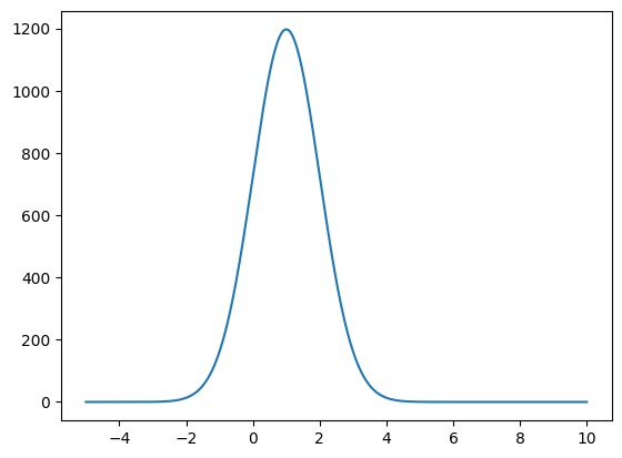
../../_images/8ffb540bc7a0b3fee890ee183e1c644e24185e037ed2e1573866e22d8b99f500.png

We can of course do better (and will see that later on, continuously improve the plots), but this is quite simple and gives us the full power of matplotlib/mplhep.

Different models#

zfit offers a selection of predefined models (and extends with models from zfit-physics that contain physics specific models such as ARGUS shaped models).

print(zfit.pdf.__all__)

print(zphysics.pdf.__all__)

To create a more realistic model, we can build some components for a mass fit with a

signal component: CrystalBall
combinatorial background: Exponential
partial reconstructed background on the left: Kernel Density Estimation

Extended tutorial on different KDEs in zfit

Shape fit#

mass_obs = zfit.Space('mass', (0, 1000))

# Signal component

mu_sig = zfit.Parameter('mu_sig', 400, 100, 600)
sigma_sig = zfit.Parameter('sigma_sig', 50, 1, 100)
alpha_sig = zfit.Parameter('alpha_sig', 200, 100, 400, floating=False)  # won't be used in the fit
npar_sig = zfit.Parameter('n sig', 4, 0.1, 30, floating=False)
signal = zfit.pdf.CrystalBall(obs=mass_obs, mu=mu_sig, sigma=sigma_sig, alpha=alpha_sig, n=npar_sig)

# combinatorial background

lam = zfit.Parameter('lambda', -0.01, -0.05, -0.0001)
comb_bkg = zfit.pdf.Exponential(lam, obs=mass_obs)

part_reco_data = np.random.normal(loc=150, scale=160, size=70_000)
part_reco = zfit.pdf.KDE1DimGrid(obs=mass_obs, data=part_reco_data)

Composing models#

We can also compose multiple models together. Here we’ll stick to one dimensional models, the extension to multiple dimensions is explained in the “custom models tutorial”.

Here we will use a SumPDF. This takes pdfs and fractions. If we provide n pdfs and:

n - 1 fracs: the nth fraction will be 1 - sum(fracs)
n fracs: no normalization attempt is done by SumPDf. If the fracs are not implicitly normalized, this can lead to bad fitting behavior if there is a degree of freedom too much

Extended tutorial on composed models, including multidimensional products

sig_frac = zfit.Parameter('sig_frac', 0.3, 0, 1)
comb_bkg_frac = zfit.Parameter('comb_bkg_frac', 0.25, 0, 1)
model = zfit.pdf.SumPDF([signal, comb_bkg, part_reco], [sig_frac, comb_bkg_frac])

In order to have a corresponding data sample, we can just create one. Since we want to fit to this dataset later on, we will create it with slightly different values. Therefore, we can use the ability of a parameter to be set temporarily to a certain value with

print(f"before: {sig_frac}")
with sig_frac.set_value(0.25):
    print(f"new value: {sig_frac}")
print(f"after 'with': {sig_frac}")

While this is useful, it does not fully scale up. We can use the zfit.param.set_values helper therefore. (Sidenote: instead of a list of values, we can also use a FitResult, the given parameters then take the value from the result)

with zfit.param.set_values([mu_sig, sigma_sig, sig_frac, comb_bkg_frac, lam], [370, 34, 0.08, 0.31, -0.0025]):
    data = model.sample(n=10_000)

plot_model(model, data);

Plotting the components is not difficult now: we can either just plot the pdfs separately (as we still can access them) or in a generalized manner by accessing the pdfs attribute:

def plot_comp_model(model, data):
    for mod, frac in zip(model.pdfs, model.params.values()):
        plot_model(mod, data, scale=frac, plot_data=False)
    plot_model(model, data)

plot_comp_model(model, data)

Now we can add legends etc. Btw, did you notice that actually, the frac params are zfit Parameters? But we just used them as if they were Python scalars and it works.

print(model.params)

Extended PDFs#

So far, we have only looked at normalized PDFs that do contain information about the shape but not about the absolute scale. We can make a PDF extended by adding a yield to it.

The behavior of the new, extended PDF does NOT change, any methods we called before will act the same. Only exception, some may require an argument less now. All the methods we used so far will return the same values. What changes is that the flag model.is_extended now returns True. Furthermore, we have now a few more methods that we can use which would have raised an error before:

get_yield: return the yield parameter (notice that the yield is not added to the shape parameters params)
ext_{pdf,integrate}: these methods return the same as the versions used before, however, multiplied by the yield
sample is still the same, but does not require the argument n anymore. By default, this will now equal to a poissonian sampled n around the yield.

The SumPDF now does not strictly need fracs anymore: if all input PDFs are extended, the sum will be as well and use the (normalized) yields as fracs

The preferred way to create an extended PDf is to use extended=yield in the PDF constructor.

Alternatively, one can use extended_pdf = pdf.create_extended(yield). (Since this relies on copying the PDF, which may does not work for different reasons, there is also a pdf.set_yield(yield) method that sets the yield in-place. This won’t lead to ambiguities, as everything is supposed to work the same.)

yield_model = zfit.Parameter('yield_model', 10000, 0, 20000, step_size=10)
model_ext = model.create_extended(yield_model)

alternatively, we can create the models as extended and sum them up

sig_yield = zfit.Parameter('sig_yield', 2000, 0, 10000, step_size=1)
sig_ext = signal.create_extended(sig_yield)

comb_bkg_yield = zfit.Parameter('comb_bkg_yield', 6000, 0, 10000, step_size=1)
comb_bkg_ext = comb_bkg.create_extended(comb_bkg_yield)

part_reco_yield = zfit.Parameter('part_reco_yield', 2000, 0, 10000, step_size=1)
part_reco.set_yield(
    part_reco_yield)  # unfortunately, `create_extended` does not work here. But no problem, it won't change anything.
part_reco_ext = part_reco

model_ext_sum = zfit.pdf.SumPDF([sig_ext, comb_bkg_ext, part_reco_ext])

Loss#

A loss combines the model and the data, for example to build a likelihood. Furthermore, it can contain constraints, additions to the likelihood. Currently, if the Data has weights, these are automatically taken into account.

nll_gauss = zfit.loss.UnbinnedNLL(gauss, data_normal)

The loss has several attributes to be transparent to higher level libraries. We can calculate the value of it using value.

nll_gauss.value()

Notice that due to graph building, this will take significantly longer on the first run. Rerun the cell above and it will be way faster.

Furthermore, the loss also provides a possibility to calculate the gradients or, often used, the value and the gradients.

nll_gauss.gradient()

We can access the data and models (and possible constraints)

nll_gauss.model

nll_gauss.data

nll_gauss.constraints

Similar to the models, we can also get the parameters via get_params.

nll_gauss.get_params()

Extended loss#

More interestingly, we can now build a loss for our composite sum model using the sampled data. Since we created an extended model, we can now also create an extended likelihood, taking into account a Poisson term to match the yield to the number of events.

nll = zfit.loss.ExtendedUnbinnedNLL(model_ext_sum, data)

nll.get_params()

Minimization#

While a likelihood is interesting, we usually want to minimize it. Therefore, we can use the minimizers in zfit, most notably Minuit, a wrapper around the iminuit minimizer.

The philosophy is to create a minimizer instance that is mostly stateless, e.g. does not remember the position.

Given that iminuit provides us with a very reliable and stable minimizer, it is usually recommended to use this. Others are implemented as well and could easily be wrapped, however, the convergence is usually not as stable.

Minuit has a few options:

tol: the Estimated Distance to Minimum (EDM) criteria for convergence (default 1e-3)
verbosity: between 0 and 10, 5 is normal, 7 is verbose, 10 is maximum
gradient: if True, uses the Minuit numerical gradient instead of the TensorFlow gradient. This is usually more stable for smaller fits; furthermore, the TensorFlow gradient can (experience based) sometimes be wrong. Using "zfit" uses the TensorFlow gradient.

minimizer = zfit.minimize.Minuit()
# minimizer = zfit.minimize.NLoptLBFGSV1()

Other minimizers#

There are a couple of other minimizers, such as SciPy, NLopt that are wrapped and can be used.

They all provide a highly standardize interface, good initial values and non-ambiguous docstring, i.e. every method has its own docstring.

When to stop: a crucial problem is the question of convergence. iminuit has the EDM, a comparably reliable metric. Other minimizers in zfit use the same stopping criteria, to be able to compare results, but that is often very inefficienc: many minimizer do not use the Hessian, required for the EDM, internally, or do not provide it. This means, the Hessian has to be calculated separately (expensive!). Better stopping criteria ideas are welcome!

help(zfit.minimize.ScipyNewtonCGV1.__init__)

print(zfit.minimize.__all__)

For the minimization, we can call minimize, which takes a

loss as we created above
optionally: the parameters to minimize

By default, minimize uses all the free floating parameters (obtained with get_params). We can also explicitly specify which ones to use by giving them (or better, objects that depend on them) to minimize; note however that non-floating parameters, even if given explicitly to minimize won ‘t be minimized.

iminuit compatibility#

As a sidenote, a zfit loss provides the same API as required by iminuit. Therefore, we can also directly invoke iminuit and use it.

The advantage can be that iminuit offers a few things out-of-the-box, like contour drawings, which zfit does not. Disadvantage is that the zfit worflow is exited.

import iminuit

iminuit_min = iminuit.Minuit(nll, nll.get_params())
# iminuit_min.migrad()  # this fails sometimes, as iminuit doesn't use the limits and is therefore unstable

result = minimizer.minimize(nll)

plot_comp_model(model_ext_sum, data)

Fit result#

The result of every minimization is stored in a FitResult. This is the last stage of the zfit workflow and serves as the interface to other libraries. Its main purpose is to store the values of the fit, to reference to the objects that have been used and to perform (simple) uncertainty estimation.

Extended tutorial on the FitResult

print(result)

This gives an overview over the whole result. Often we’re mostly interested in the parameters and their values, which we can access with a params attribute.

print(result.params)

This is a dict which stores any knowledge about the parameters and can be accessed by the parameter (object) itself:

result.params[mu_sig]

‘value’ is the value at the minimum. To obtain other information about the minimization process, result contains more attributes:

valid: whether the result is actually valid or not (most important flag to check)
fmin: the function minimum
edm: estimated distance to minimum
info: contains a lot of information, especially the original information returned by a specific minimizer
converged: if the fit converged

result.fmin

Info provides additional information on the minimization, which can be minimizer dependent. For example, if iminuit was used, the instance can be retrieved.

print(result.info['minuit'])  # the actual instance used in minimization

Estimating uncertainties#

The FitResult has mainly two methods to estimate the uncertainty:

a profile likelihood method (like MINOS)
Hessian approximation of the likelihood (like HESSE)

When using Minuit, this uses (currently) its own implementation. However, zfit has its own implementation, which can be invoked by changing the method name.

Hesse also supports the corrections for weights.

We can explicitly specify which parameters to calculate, by default it does for all.

result.hesse(name='hesse')

# result.hesse(method='hesse_np', name='numpy_hesse')
# result.hesse(method='minuit_hesse', name='iminuit_hesse')

We get the result directly returned. This is also added to result.params for each parameter and is nicely displayed with an added column

print(result.params)

errors, new_result = result.errors(params=[sig_yield, part_reco_yield, mu_sig],
                                   name='errors')  # just using three, but we could also omit argument -> all used

errorszfit, new_result_zfit = result.errors(params=[sig_yield, part_reco_yield, mu_sig], method='zfit_errors', name='errorszfit')

print(errors)

print(result)

What is ‘new_result’?#

When profiling a likelihood, such as done in the algorithm used in errors, a new minimum can be found. If this is the case, this new minimum will be returned, otherwise new_result is None. Furthermore, the current result would be rendered invalid by setting the flag valid to False. Note: this behavior only applies to the zfit internal error estimator.

We can also access the covariance matrix of the parameters

result.covariance()

Bonus: serialization#

Human-readable serialization is experimentally supported in zfit. zfit aims to follow the HS3 standard, which is currently in development.

Extended tutorial on serialization

model.to_dict()

gauss.to_yaml()

zfit.hs3.dumps(nll)

End of zfit#

This is where zfit finishes and other libraries take over.

Beginning of hepstats#

hepstats is a library containing statistical tools and utilities for high energy physics. In particular you do statistical inferences using the models and likelhoods function constructed in zfit.

Short example: let’s compute for instance a confidence interval at 68 % confidence level on the mean of the gaussian defined above.

from hepstats.hypotests import ConfidenceInterval
from hepstats.hypotests.calculators import AsymptoticCalculator
from hepstats.hypotests.parameters import POIarray

calculator = AsymptoticCalculator(input=result, minimizer=minimizer)

value = result.params[mu_sig]["value"]
error = result.params[mu_sig]["hesse"]["error"]

mean_scan = POIarray(mu_sig, np.linspace(value - 1.5 * error, value + 1.5 * error, 10))

ci = ConfidenceInterval(calculator, mean_scan)

ci.interval()

from utils import one_minus_cl_plot

ax = one_minus_cl_plot(ci)
ax.set_xlabel("mean")

There will be more of hepstats later.