Bayesian Inference

A concise introduction to modern Bayesian inference in zfit covering essential features:

• Prior specification: Define prior beliefs about parameters before seeing data

• MCMC sampling: Use Markov Chain Monte Carlo (emcee) to sample from posterior distributions

• Convergence diagnostics: Monitor R̂ (Gelman-Rubin statistic) and ESS (Effective Sample Size)

• ArviZ integration: Advanced diagnostics and visualization tools

• Posterior analysis: Extract credible intervals, means, and covariances

---

from __future__ import annotations

import os

os.environ["ZFIT_DISABLE_TF_WARNINGS"] = "1"  # Suppress TensorFlow warnings
os.environ["CUDA_VISIBLE_DEVICES"] = "-1"  # disable GPU

import matplotlib.pyplot as plt
import numpy as np
import zfit

np.random.seed(42)

Bayesian Analysis Fundamentals

Bayesian inference uses Bayes’ theorem to update beliefs about parameters given data:

\[P(\theta | data) = \frac{P(data | \theta) \cdot P(\theta)}{P(data)}\]

Where:

• P(θ|data): Posterior - updated beliefs after seeing data

• P(data|θ): Likelihood - probability of observing data given parameters

• P(θ): Prior - initial beliefs about parameters before seeing data

Priors encode domain knowledge or express ignorance. Unlike frequentist methods that treat parameters as fixed unknowns, Bayesian analysis treats them as random variables with probability distributions.

# Available prior distributions in zfit
uniform_prior = zfit.prior.Uniform(lower=0, upper=10)
normal_prior = zfit.prior.Normal(mu=5.0, sigma=1.0)
gamma_prior = zfit.prior.Gamma(alpha=2.0, beta=1.0)
half_normal_prior = zfit.prior.HalfNormal(sigma=0.5)
poisson_prior = zfit.prior.Poisson(lam=3.0)
exponential_prior = zfit.prior.Exponential(lam=2.0)
student_t_prior = zfit.prior.StudentT(ndof=3, mu=0.0, sigma=1.0)

1. Model Setup with Priors

Signal+background model with physics-motivated priors:

• μ: Uniform around expected peak location

• σ: HalfNormal (positive, favors smaller widths)

• λ: Normal around typical decay rate

• Yields: Normal based on expected counts

Priors can be set during creation or modified later:

# Setting and changing priors
param = zfit.Parameter("demo", 1.0, lower=0.0, upper=5.0)
print(f"Initial prior: {param.prior}")
param.set_prior(zfit.prior.Normal(mu=2.0, sigma=0.5))
print(f"Updated prior: {param.prior}")
param.set_prior(zfit.prior.Exponential(lam=1.0))
print(f"Exponential prior: {param.prior}")
param.set_prior(None)  # Remove prior
print(f"Removed prior: {param.prior}")

Initial prior: None

Updated prior: Normal(name='None')

Exponential prior: Exponential(name='None')

Removed prior: None

# Define observable and parameters with priors
obs = zfit.Space("mass", 4.0, 6.0)

# Signal parameters
mu = zfit.Parameter("mu", 5.1, 4.5, 5.5, prior=zfit.prior.Uniform(lower=4.8, upper=5.2))
sigma = zfit.Parameter("sigma", 0.2, 0.05, 0.3, prior=zfit.prior.HalfNormal(sigma=0.1))
lambda_bkg = zfit.Parameter("lambda_bkg", -1.2, -3.0, 0.0, prior=zfit.prior.Normal(mu=-1.0, sigma=0.5))

# Yield parameters
n_sig = zfit.Parameter("n_sig", 900, 0, 5000, prior=zfit.prior.Normal(mu=1000, sigma=100))
n_bkg = zfit.Parameter("n_bkg", 600, 0, 2000, prior=zfit.prior.Normal(mu=500, sigma=50))

# Create model
signal = zfit.pdf.Gauss(obs=obs, mu=mu, sigma=sigma, extended=n_sig)
background = zfit.pdf.Exponential(obs=obs, lambda_=lambda_bkg, extended=n_bkg)
model = zfit.pdf.SumPDF([signal, background])

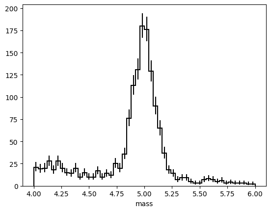
# Generate synthetic data from the model
true_params = {mu: 5.0, sigma: 0.1, lambda_bkg: -1.0, n_sig: 1000, n_bkg: 500}
data = model.sample(n=1500, params=true_params)
data.to_binned(50).to_hist().plot(label="Data", color="black", histtype="step")

[StairsArtists(stairs=<matplotlib.patches.StepPatch object at 0x7e2c04fcf200>, errorbar=<ErrorbarContainer object of 3 artists>, legend_artist=<ErrorbarContainer object of 3 artists>)]

# Create loss function
nll = zfit.loss.ExtendedUnbinnedNLL(model=model, data=data)

3. MCMC Sampling

MCMC constructs a Markov chain to sample from the posterior. The emcee ensemble sampler uses multiple walkers for efficiency and affine invariance.

Key parameters:

• nwalkers: Ensemble size, typically ≥ 2× parameters

• n_warmup: Burn-in steps to reach stationarity, 200-500 for simple models, more for complex ones

• n_samples: Production samples, 1000+ for final results, 100-500 for testing

# Initialize MCMC sampler
sampler = zfit.mcmc.EmceeSampler(nwalkers=32, verbosity=8)  # 8 shows progressbar

# Sample from posterior
posterior = sampler.sample(
    loss=nll,
    n_samples=500,  # Reduced for tutorial speed
    n_warmup=200,
)

Running burn-in phase with 200 steps...

Running production phase with 500 steps...

4. Results Analysis

The posterior provides parameter estimates and convergence diagnostics:

• R̂: Gelman-Rubin statistic, convergence metric comparing within-chain to between-chain variance (≤ 1.1 indicates good convergence)

• ESS: Effective sample size accounting for autocorrelation (higher = better sampling efficiency)

• Credible intervals: Bayesian confidence intervals

• Methods: mean(), std(), credible_interval(), get_samples()

print(posterior)

PosteriorSamples

 from
<ExtendedUnbinnedNLL model=[<zfit.<class 'zfit.models.functor.SumPDF'>  params=[Composed_autoparam_40, Composed_autoparam_41]] data=[<zfit.Data: Data obs=('mass',) shape=(1500, 1)>] constraints=[]> 
with
EmceeSampler(name='EmceeSampler')

╒═════════╤═════════════╤═════════╤═══════════╤═══════════════════════════════════════╕
│  valid  │  converged  │  max R̂  │  min ESS  │   total samples | warmup | per walker │
╞═════════╪═════════════╪═════════╪═══════════╪═══════════════════════════════════════╡
│  

True

   │    

True

     │ 1.0182  │   13836   │           16000 |    200 |        500 │
╘═════════╧═════════════╧═════════╧═══════════╧═══════════════════════════════════════╛

Parameters

parameter        mean        std                    95% CI       R̂    ESS
-----------  --------  ---------  ------------------------  ------  -----
n_sig        990.1117  ± 33.0327  [  927.1198,  1057.1145]  1.0140  13836
n_bkg        509.7380  ± 23.9976  [  465.3629,   559.2928]  1.0120  16911
mu             4.9969   ± 0.0034  [    4.9901,     5.0035]  1.0130  13893
sigma          0.0982   ± 0.0031  [    0.0924,     0.1043]  1.0100  14288
lambda_bkg    -0.9974   ± 0.0906  [   -1.1745,    -0.8256]  1.0180  17974

Sampler: EmceeSampler with 32 walkers

# Extract parameter estimates
for param in model.get_params():
    mean_val = posterior.mean(param)
    std_val = posterior.std(param)
    print(f"{param.name}: {mean_val:.4f} ± {std_val:.4f}")

print("\n90% credible intervals:")
for param in model.get_params():
    lower, upper = posterior.credible_interval(param, alpha=0.1)
    print(f"{param.name}: [{lower:.4f}, {upper:.4f}]")

n_sig: 990.1117 ± 33.0327

n_bkg: 509.7380 ± 23.9976

mu: 4.9969 ± 0.0034

sigma: 0.0982 ± 0.0031

lambda_bkg: -0.9974 ± 0.0906

90% credible intervals:

n_sig: [937.2390, 1045.3623]

n_bkg: [471.9161, 552.1484]

mu: [4.9912, 5.0023]

sigma: [0.0934, 0.1033]

lambda_bkg: [-1.1470, -0.8480]

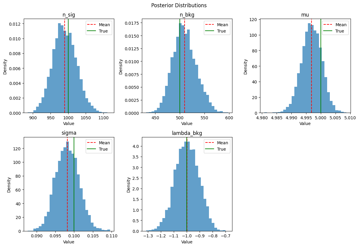
5. Visualization

Posterior plots show parameter uncertainties and compare to true values. Key insights:

• Width: Parameter uncertainty

• Shape: Non-Gaussian features

• Location: How data updated the prior

# Plot posterior distributions
fig, axes = plt.subplots(2, 3, figsize=(12, 8))
axes = axes.flatten()

for i, param in enumerate(model.get_params()):
    if i < len(axes):
        samples = posterior.get_samples(param)
        axes[i].hist(samples, bins=30, alpha=0.7, density=True)
        axes[i].axvline(posterior.mean(param), color="red", linestyle="--", label="Mean")
        axes[i].axvline(true_params[param], color="green", linestyle="-", label="True")
        axes[i].set_title(f"{param.name}")
        axes[i].set_xlabel("Value")
        axes[i].set_ylabel("Density")
        axes[i].legend()

# Remove empty subplot
if len(model.get_params()) < len(axes):
    fig.delaxes(axes[-1])

plt.tight_layout()
plt.suptitle("Posterior Distributions", y=1.02)
plt.show()

# ArviZ integration for advanced diagnostics
import arviz as az

# Convert to ArviZ InferenceData format
idata = posterior.to_arviz()

# Print summary with R-hat and ESS
summary = az.summary(idata)
print(summary)

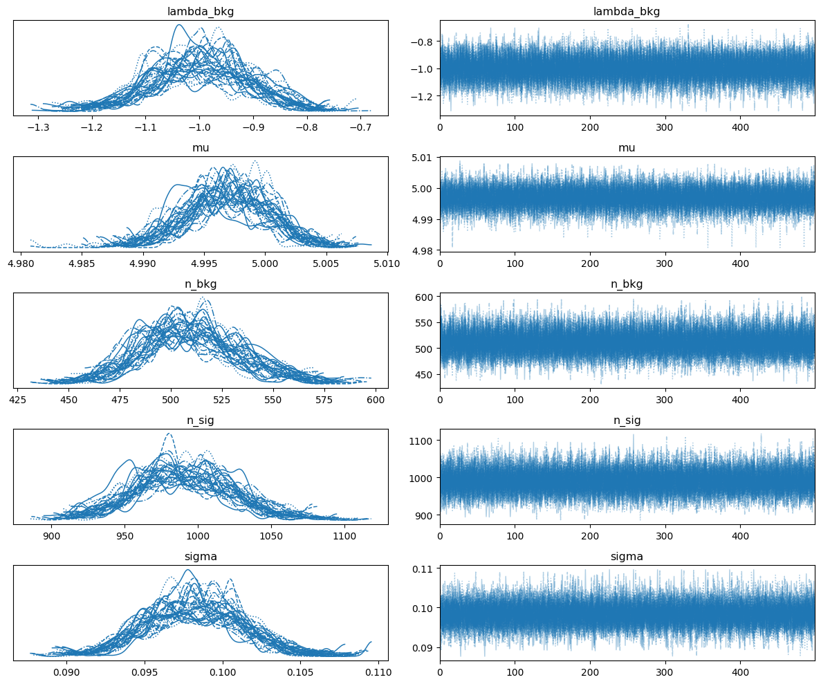
# Plot trace plots
az.plot_trace(idata, compact=True)
plt.tight_layout()
plt.show()

# Check R-hat values
rhat = az.rhat(idata)
print("\nR-hat values (should be ≤ 1.1):")
for var in rhat.data_vars:
    print(f"{var}: {float(rhat[var]):.3f}")

# Effective sample size
ess = az.ess(idata)
print("\nEffective sample sizes:")
for var in ess.data_vars:
    print(f"{var}: {float(ess[var]):.0f}")

               mean      sd   hdi_3%   hdi_97%  mcse_mean  mcse_sd  ess_bulk  \
lambda_bkg   -0.997   0.091   -1.168    -0.831      0.001    0.001   17974.0   
mu            4.997   0.003    4.990     5.003      0.000    0.000   13893.0   
n_bkg       509.738  23.998  466.543   556.719      0.185    0.133   16911.0   
n_sig       990.112  33.034  926.415  1050.127      0.278    0.176   13836.0   
sigma         0.098   0.003    0.093     0.104      0.000    0.000   14288.0   

            ess_tail  r_hat  
lambda_bkg   14211.0   1.02  
mu           15934.0   1.01  
n_bkg        15781.0   1.01  
n_sig        15375.0   1.01  
sigma        15120.0   1.01  

R-hat values (should be ≤ 1.1):

lambda_bkg: 1.018

mu: 1.013

n_bkg: 1.012

n_sig: 1.014

sigma: 1.010

Effective sample sizes:

lambda_bkg: 17974

mu: 13893

n_bkg: 16911

n_sig: 13836

sigma: 14288

After the fit is before the fit

# 1. Posterior to prior for hierarchical modeling
mu_posterior_prior = posterior.as_prior(mu)
print(f"Created KDE prior from posterior: {mu_posterior_prior}")

Created KDE prior from posterior: KDE(name='mu_posterior_prior')

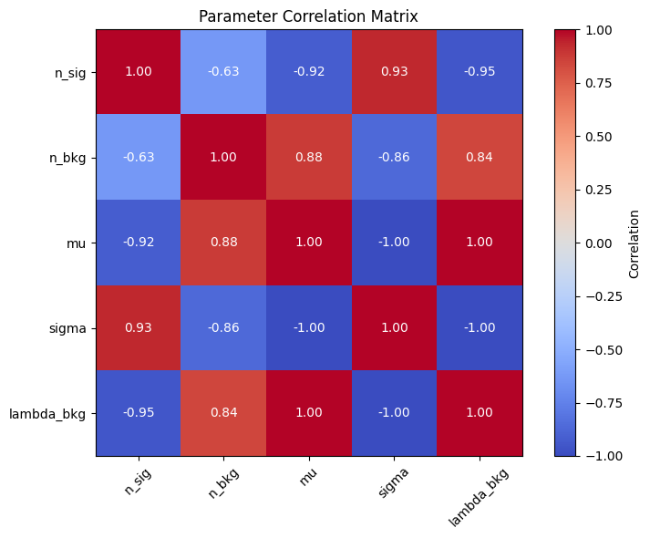
# Covariance matrix and correlations
cov_matrix = posterior.covariance()
param_names = [p.name for p in model.get_params()]
corr_matrix = np.corrcoef(cov_matrix)

plt.figure(figsize=(8, 6))
plt.imshow(corr_matrix, cmap="coolwarm", vmin=-1, vmax=1)
plt.colorbar(label="Correlation")
plt.xticks(range(len(param_names)), param_names, rotation=45)
plt.yticks(range(len(param_names)), param_names)
plt.title("Parameter Correlation Matrix")
for i in range(len(param_names)):
    for j in range(len(param_names)):
        plt.text(
            j,
            i,
            f"{corr_matrix[i, j]:.2f}",
            ha="center",
            va="center",
            color="white" if abs(corr_matrix[i, j]) > 0.5 else "black",
        )
plt.tight_layout()
plt.show()

# Context manager for setting parameters to posterior means, same as FitResult
original_mu = mu.value()

with posterior:
    posterior_mu = mu.value()

print(f"Original mu: {original_mu:.4f}")
print(f"Posterior mean mu: {posterior_mu:.4f}")
print(f"After context: {mu.value():.4f}")

Original mu: 5.1000

Posterior mean mu: 4.9969

After context: 5.1000